The Synthetic Control Method in Stata

Did Proposition 99 cut smoking in California?

−19.00ATT · packs per capita / yr

0.974pre-treatment R² (synth2)

0.026in-space placebo p-value

Carlos Mendez

Nagoya University (GSID)

October 5, 2026

The Tension

Act I

Smoking was falling everywhere, so did the tax change anything?

In 1988, California voters passed Proposition 99, effective January 1989. It raised the cigarette tax by 25 cents per pack. It also funded anti-smoking education.

Yet cigarette sales were already falling nationwide. In California, the decline began in the late 1970s. What would California have done without the law?

A simple before-and-after comparison confounds the policy with a trend that pushed sales down everywhere. This is the central problem of policy evaluation with a single treated unit. We cannot simply compare California before and after 1989. Secular trends, such as rising health awareness and federal regulation, were already lowering sales across the country. We therefore need a credible counterfactual: a California that never passed Proposition 99.

A raw comparison hints at an effect, but the comparator is crude

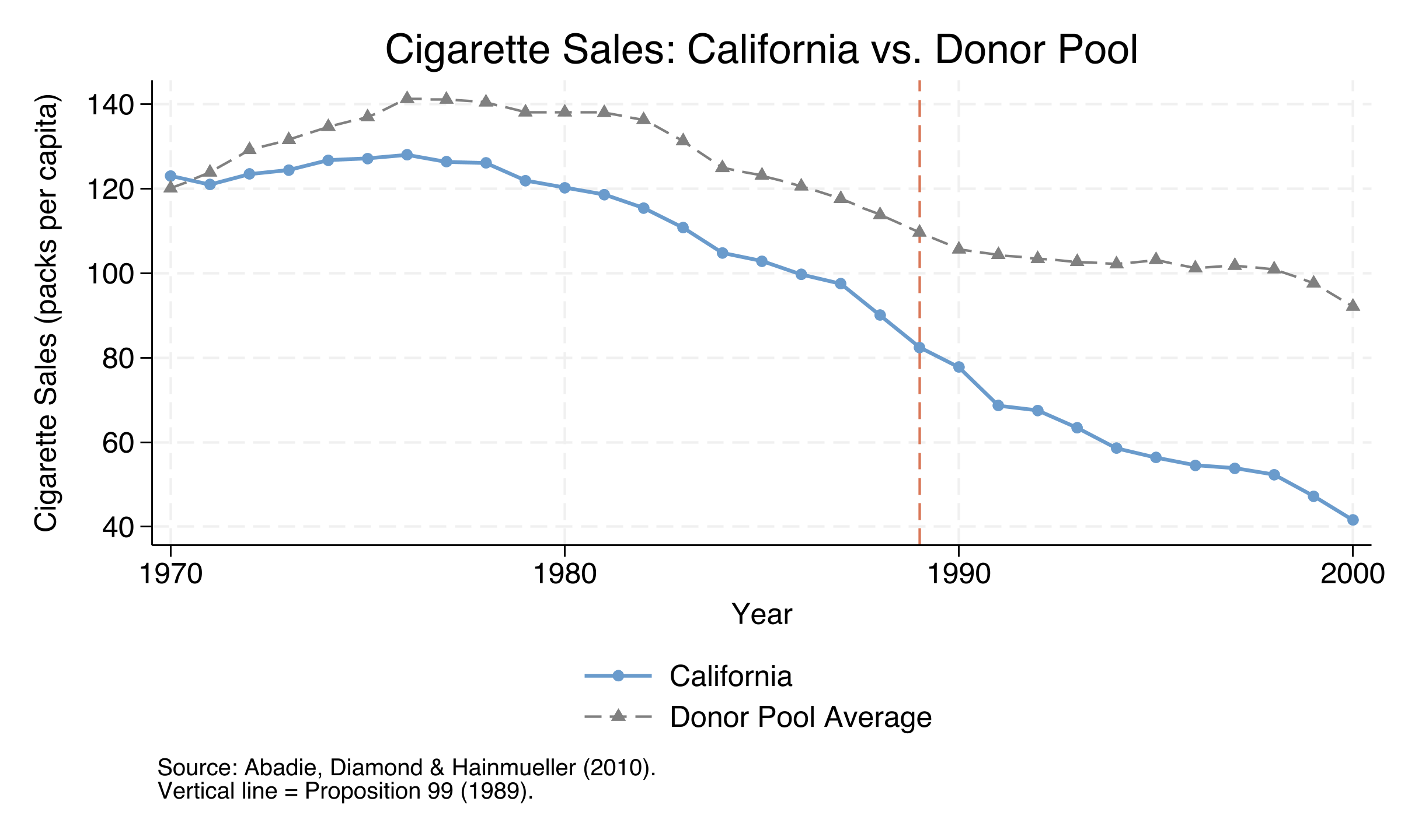
Cigarette sales per capita, 1970–2000: California (solid blue) versus the unweighted average of 38 control states (dashed gray). The orange line marks Proposition 99 (1989).

California starts close to the donor average in 1970. The gap then widens through the 1970s and stays near 20 packs for most of the 1980s. By 1988, California sold 90.1 packs per capita against a donor average of 113.8, already 23.72 packs below it before the law. The unweighted average also gives equal weight to New Hampshire and Utah, which average 213 and 64 packs per capita over 1970–2000. Their smoking levels are very different from those of California. We need an optimal weighted comparator, and that comparator is the synthetic control.

Where we are going

• The lab: a 39-state, 31-year panel and the ATT estimand
• Build “synthetic California” with synth2, a weighted blend of donor states
• Three inference tools: in-space placebo, in-time placebo, and leave-one-out
• The lesson: prefer a transparent counterfactual to an untestable parallel-trends assumption

The Investigation

Act II

The lab: 39 states × 31 years, one treated unit, the ATT

• Outcome: cigsale, cigarette sales per capita (packs)
• Treatment: Proposition 99, California only, from 1989
• Predictors: log GDP per capita, share aged 15–24, retail price, beer, and cigsale in 1975, 1980, and 1988

Strongly balanced panel: 1,209 observations, 19 pre-treatment years, and 12 post-treatment years. The estimand is the ATT for California, the one treated unit, not the ATE.

With a single treated unit and aggregate data, the parallel-trends assumption of difference-in-differences is hard to test. SCM instead builds an explicit counterfactual, so we can see the quality of the match in the pre-treatment period. California is state == 3 in the data.

SCM builds a counterfactual by matching pre-treatment predictors

\[\min_{W} \sum_{m=1}^{M} v_m \left( X_{1m} - \sum_{j=2}^{J+1} w_j X_{jm} \right)^2\]

We pick donor weights \(w_j \ge 0\) that sum to one and match the predictors \(X_{1m}\) of California. The weights \(v_m\) set how much each predictor matters. The solution is the closest feasible blend of donors.

The synthetic control is a convex combination of real states, so it never extrapolates beyond the donor pool.

This is a nested optimization. The outer problem picks the V-weights to minimize the pre-1989 prediction error of the outcome. These weights set how much each predictor counts in the matching distance. The inner problem picks the W-weights, the donor shares, that minimize the weighted predictor distance. The nonnegativity and sum-to-one constraints keep the synthetic control interpretable and limit overfitting.

The treatment effect is the gap between actual and synthetic California

\[\hat{\tau}_t = Y_{1t} - \sum_{j=2}^{J+1} w_j^* Y_{jt}\]

The effect in year \(t\) is actual minus synthetic sales. A negative \(\hat{\tau}_t\) means that the law lowered sales. Each year from 1989 to 2000 yields one such gap.

Identification rests on good pre-treatment fit, no interference, no anticipation, and no donor contamination; only the fit is directly visible in the data.

The ATT is the mean of these yearly gaps over 1989–2000. Unlike difference-in-differences, the method does not ask us to accept parallel trends on faith. If the synthetic control tracks California closely before 1989, the later divergence is a credible estimate of the effect. No interference means that Proposition 99 did not change sales in other states. No anticipation means that sales in California did not respond before 1989. No donor contamination means that the donor states adopted no similar programs during the sample period. Good fit means that the synthetic control reproduces the pre-1989 path.

One synth2 call fits the baseline synthetic control

synth2 cigsale lnincome age15to24 retprice beer ///
    cigsale(1988) cigsale(1980) cigsale(1975), ///
    trunit(3) trperiod(1989) xperiod(1980(1)1988) nested allopt

trunit(3) = California · trperiod(1989) = treatment year · nested = outer V / inner W · allopt = multiple starts to avoid local optima.

The specification uses seven predictors. Four economic and demographic variables are averaged over 1980–1988, and cigarette sales enter at three anchor years before treatment (1975, 1980, and 1988). The nested allopt combination is slower, but it lowers the risk of a spurious local optimum in the search over the V-weights. It is a careful choice, not a gold standard.

Synthetic California tracks the pre-1989 path closely, but not exactly

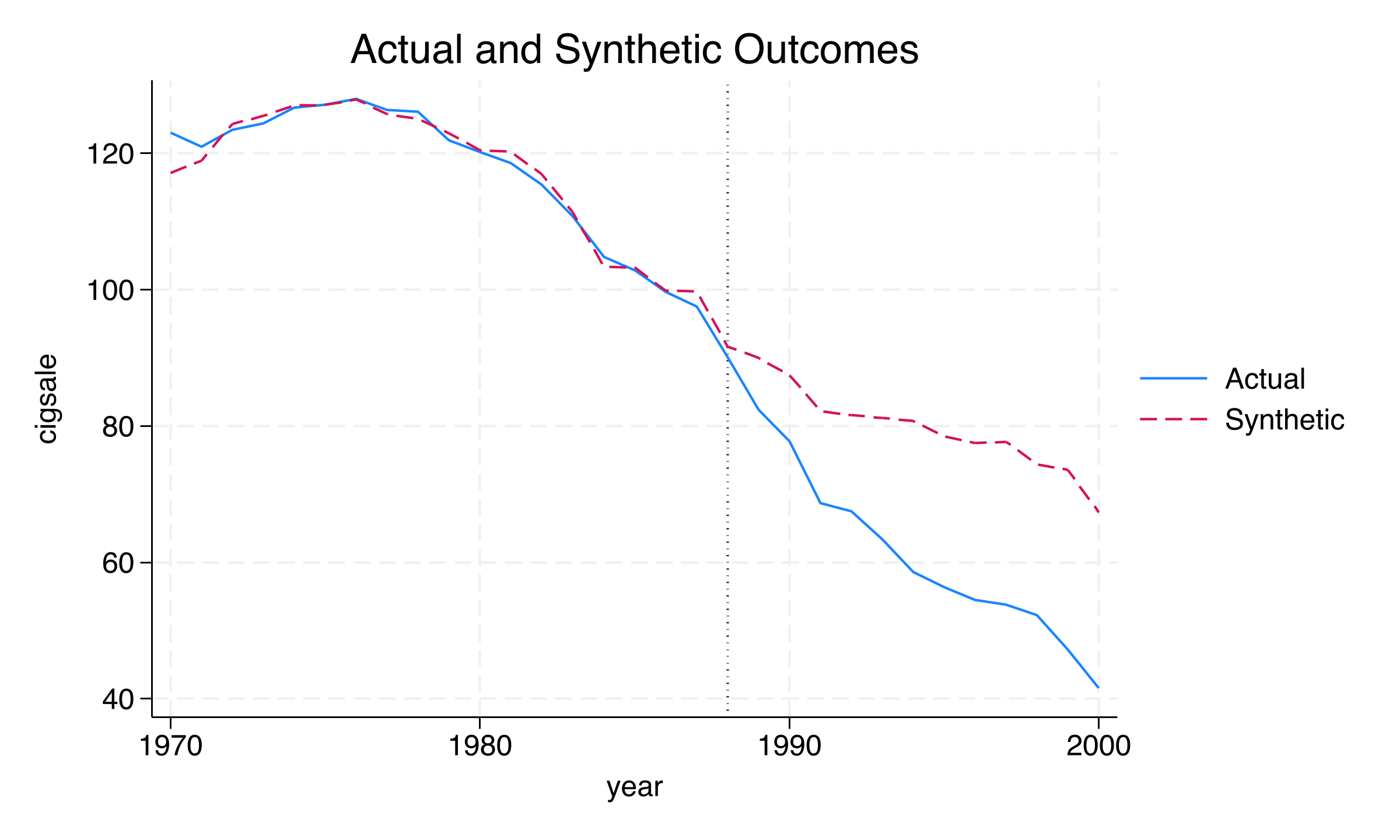
Actual versus synthetic California, 1970–2000: close before 1989 apart from 1970, then a widening gap.

The synth2 command reports an R² of 0.974 and an RMSE of 1.756 packs over the 19 pre-treatment years. Its R² divides by the variation of the synthetic series; the conventional R² with the same weights is 0.976. The fit is close but not exact: the largest pre-period gap is 5.88 packs, in 1970, and the later gaps are much smaller. This close match makes it unlikely that the post-1989 divergence merely continues a pre-existing difference.

Age 15–24 and 1975 sales dominate the V-weights, but V is fragile

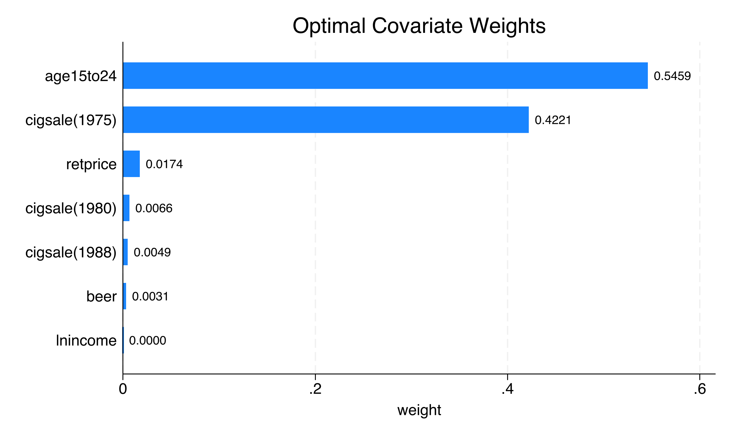
Predictor (V-matrix) weights: how much each predictor counts in the matching distance.

The dominant V-weights are age 15–24 (0.546) and cigsale(1975) (0.422), while log GDP per capita gets essentially zero weight. These weights are fragile, because V is poorly identified. The placebo refit of the same model gives age 15–24 only 0.002 and cigsale(1975) 0.768, while the donor weights barely change. We should therefore read V as one of many near-equivalent solutions, not as a ranking of what matters. In the baseline fit, six of the seven predictors are closely matched, and five biases are below 0.3%. Log GDP per capita is the exception: its −2.16% bias compares logarithms, so synthetic California falls short by 0.22 log points, a GDP per capita about 20% lower. The simple average of the controls misses 1988 sales by 26.3%, against 1.74% for the synthetic control.

Synthetic California is a blend of five states, led by Utah at one-third

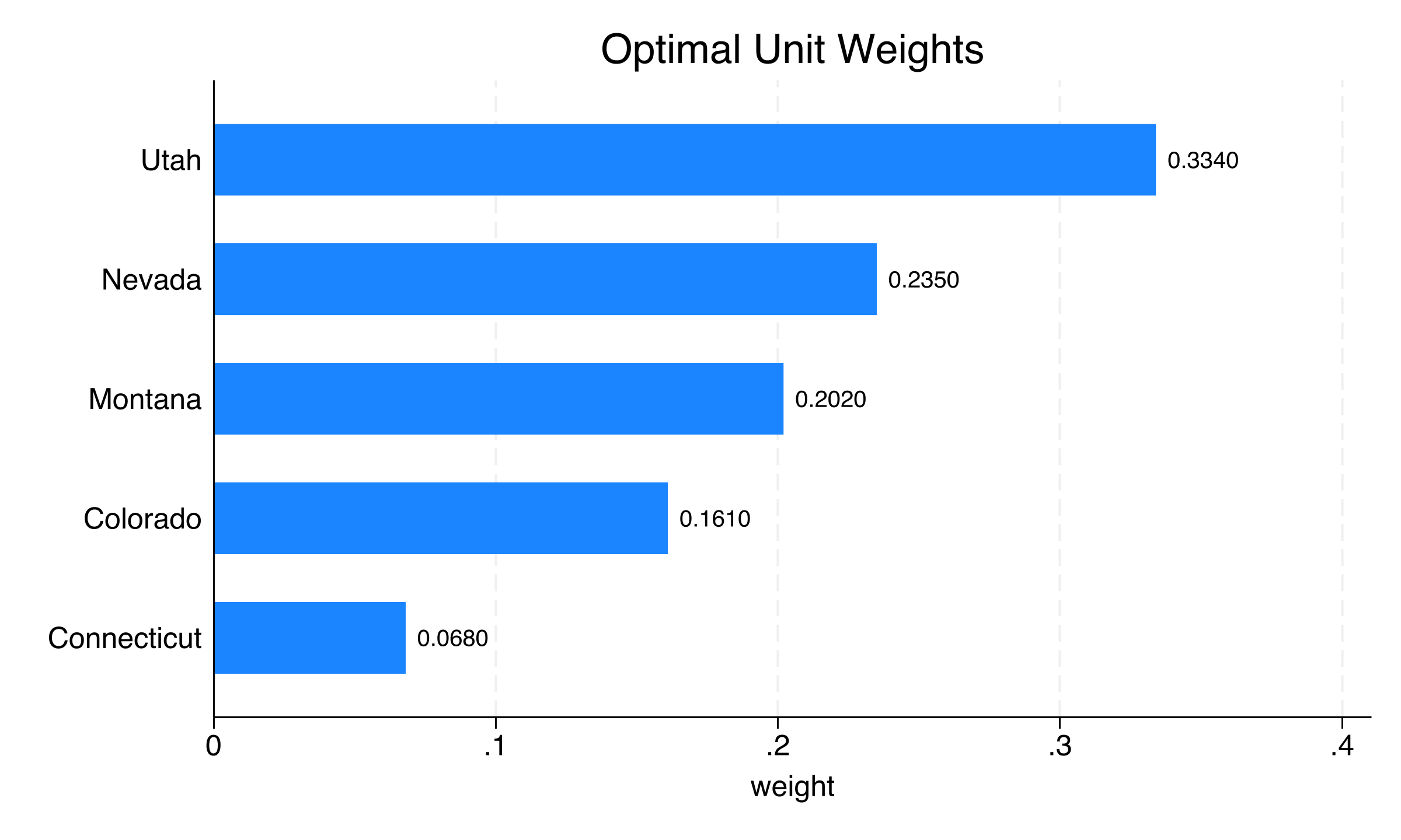
Donor weights: the five states that compose synthetic California (33 others get a reported weight of zero).

The weights are Utah 33.4%, Nevada 23.5%, Montana 20.2%, Colorado 16.1%, and Connecticut 6.8%. SCM solutions are typically sparse. The method selects the blend whose weighted predictors, including past sales, match California, not individually similar or nearby states. Low-sales Utah and high-sales Nevada, for example, bracket California. Because Utah carries a third of the weight, we later drop each donor in turn in a leave-one-out check.

By 2000, real California sold 38% fewer packs than its synthetic twin

−19.00

average ATT, packs per capita / yr (1989–2000); −7.59 in 1989 deepening to −26.37 by 1999

The effect grows over time. By 2000, actual sales in California (41.6 packs) sit 25.76 packs below the synthetic control (67.4), a reduction of 38%. With about 34 million residents, that gap implies roughly 900 million fewer packs in 2000 alone. The growing gap is consistent with cumulative behavioral change and shifting social norms. Part of the gap in 1999–2000 may also reflect Proposition 10, which raised the tax by a further 50 cents per pack in January 1999.

The gap widens through the 1990s, though not in every year

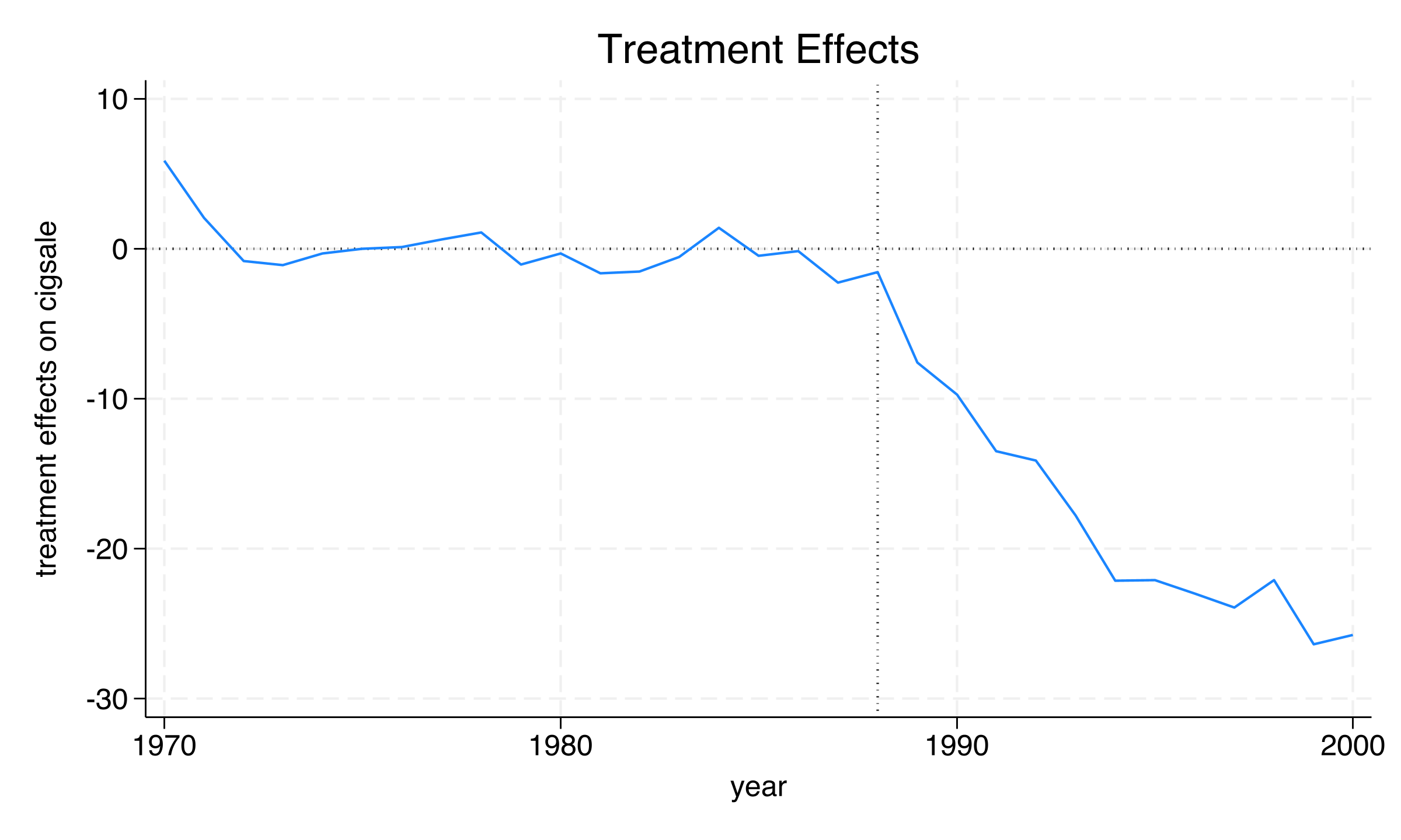
Treatment effect (actual minus synthetic California) over time; the negative gap widens after 1989.

The effect starts at −7.59 packs in 1989, reaches −26.37 by 1999, and stands at −25.76 in 2000. The path is not monotonic; for instance, the gap narrows briefly in 1998. Is the gap real, or could a state that was never treated show a gap this large by chance? Act III tests the result in three ways.

The Resolution

Act III

California has the most extreme signal-to-noise ratio of all 39 states

State	Pre MSPE	Post/Pre MSPE
California	3.17	123.5
Georgia	1.46	80.0
Virginia	2.78	79.0
Missouri	1.20	70.9

The post/pre MSPE ratio asks how much worse the fit becomes after 1989 than before. California has the highest ratio, well above the runner-up.

A genuine effect should inflate the post-treatment prediction error relative to a small pre-treatment error. California has a ratio of 123.5, well above Georgia (80.0) and Virginia (79.0). The table comes from the placebo run, which refits California with sigf(6) and without allopt. That refit has an RMSE of 1.780 (pre-MSPE 3.17), slightly worse than the baseline RMSE of 1.756. The ratio is the preferred statistic because it rewards both a large gap and a tight pre-treatment fit.

Run the placebo on every state: California is the clear outlier

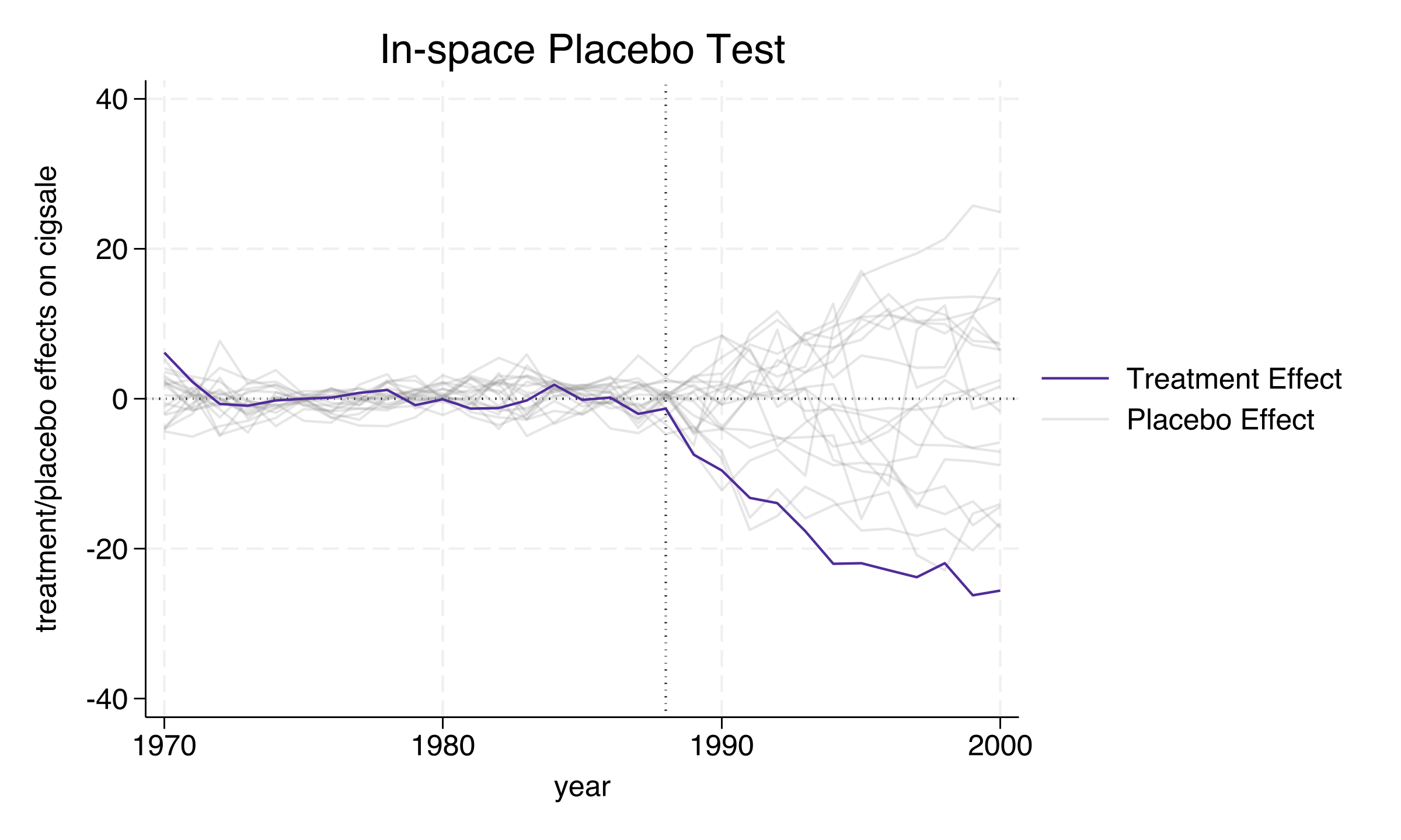
Gaps for California (purple) and the 19 placebo states retained by cut(2): the lines overlap near zero before 1989, and California falls below almost every placebo afterward.

The in-space placebo applies the same SCM to each control state, as if each had been treated in 1989. This is a permutation test: if treatment were assigned to one state at random, how often would we see a gap as large as the one for California? Rarely: by the post/pre MSPE ratio, California ranks first among all 39 units. The figure shows its path as a clear outlier among the 19 retained placebos.

Across all 39 states, a ratio this large occurs 2.6% of the time

0.026

in-space placebo p-value, all controls (1/39); p = 0.050 after the cut(2) fit filter (1/20)

Using all states, p = 1/39 = 0.026. The cut(2) filter removes the 19 states whose pre-treatment MSPE exceeds twice that of California, which leaves 20 states, California included, and p = 1/20 = 0.050. That value sits right at the conventional threshold, a mechanical consequence of having few comparison units. We report both: the unfiltered p is the less conservative of the two, while the filtered p compares California only with placebos that fit well.

Significance holds in most post-treatment years

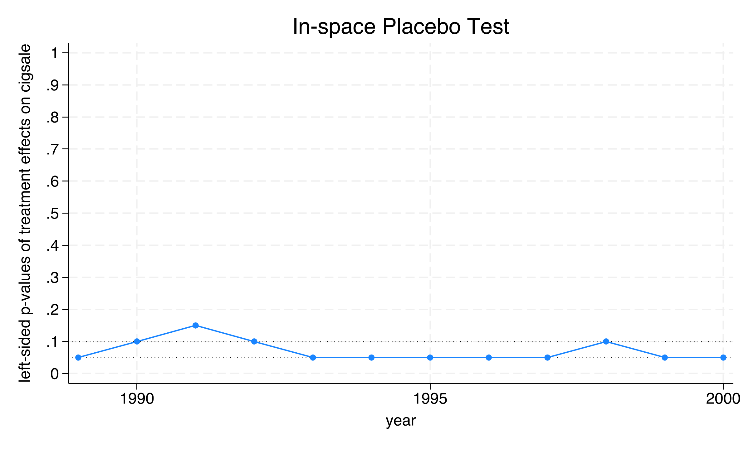
Left-sided permutation p-values over time (left-sided, because the effect is negative): p = 0.050 in most years.

Left-sided p-values are the right choice for a negative effect. They are computed on the 20 units retained by cut(2), and they equal 0.050 in 8 of 12 post-treatment years. In 1990–1992 and 1998, one or two retained placebos show a gap at least as negative as that of California, so p rises to 0.100–0.150. Effect size alone does not explain this, because the smallest gap, in 1989, still reaches p = 0.050. From 1993 onward, California is the most extreme state in every year except 1998.

A fake 1985 treatment produces much smaller gaps

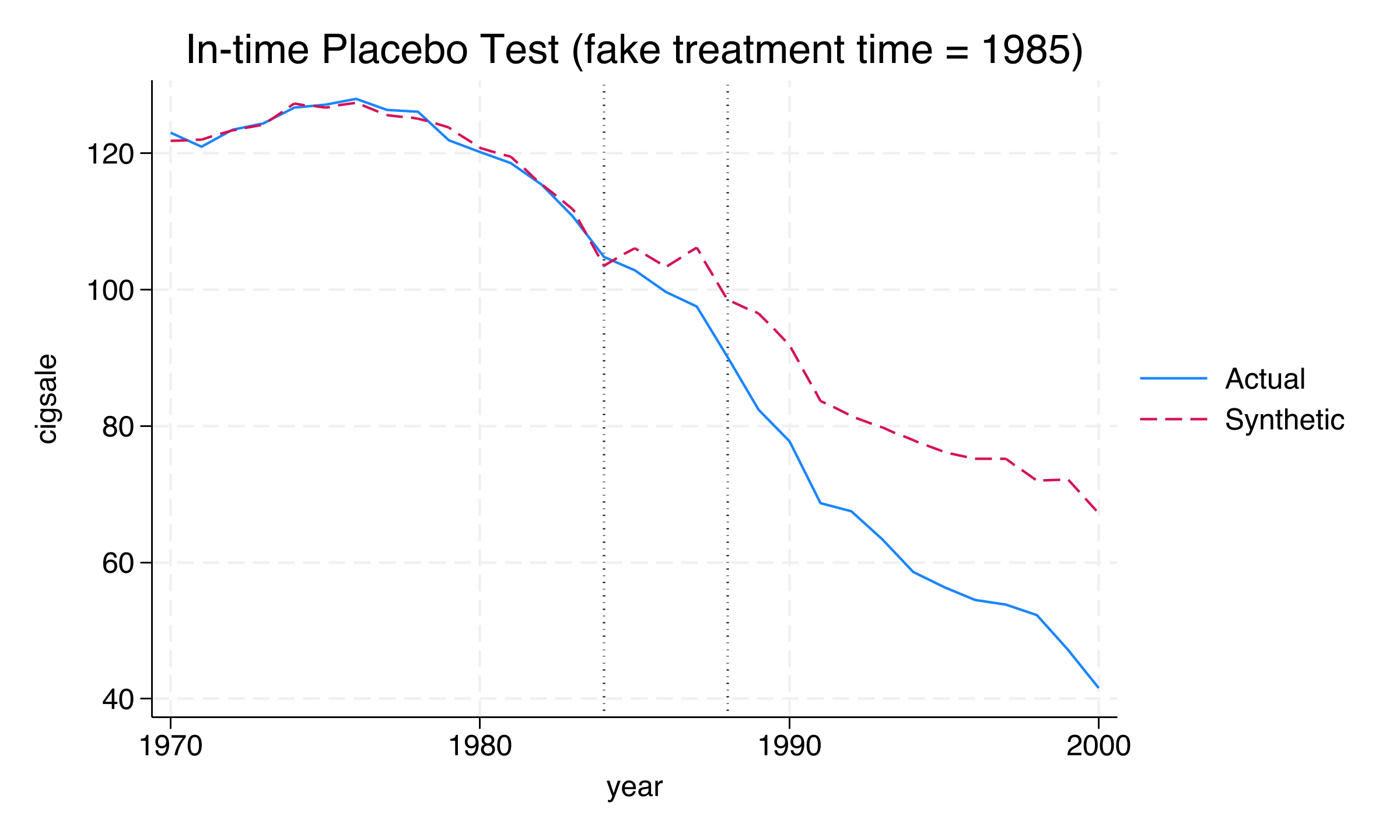
In-time placebo: actual versus synthetic California with a fake treatment in 1985. A modest gap opens during 1985–1988, and the lines split much further after the real 1989 policy.

If the design were spurious, a fake earlier date would produce an effect of similar size. Instead, the fake-period gaps (1985–1988) range from −3.33 to −8.65 packs, while the gaps from 1989 onward range from −13.97 to −25.59 packs. The fake model uses a reduced specification: covariates are averaged over 1980–1984, the 1988 lag is dropped, and the fit period is 1970–1984. The synth2 command does not print the fit of this fake-1985 model. The R² of 0.953 in the log belongs to the same reduced specification estimated with the real date 1989. The fake-period gaps are much smaller than the real ones, but they are not zero.

The gap stays modest at the fake date and grows after the real one

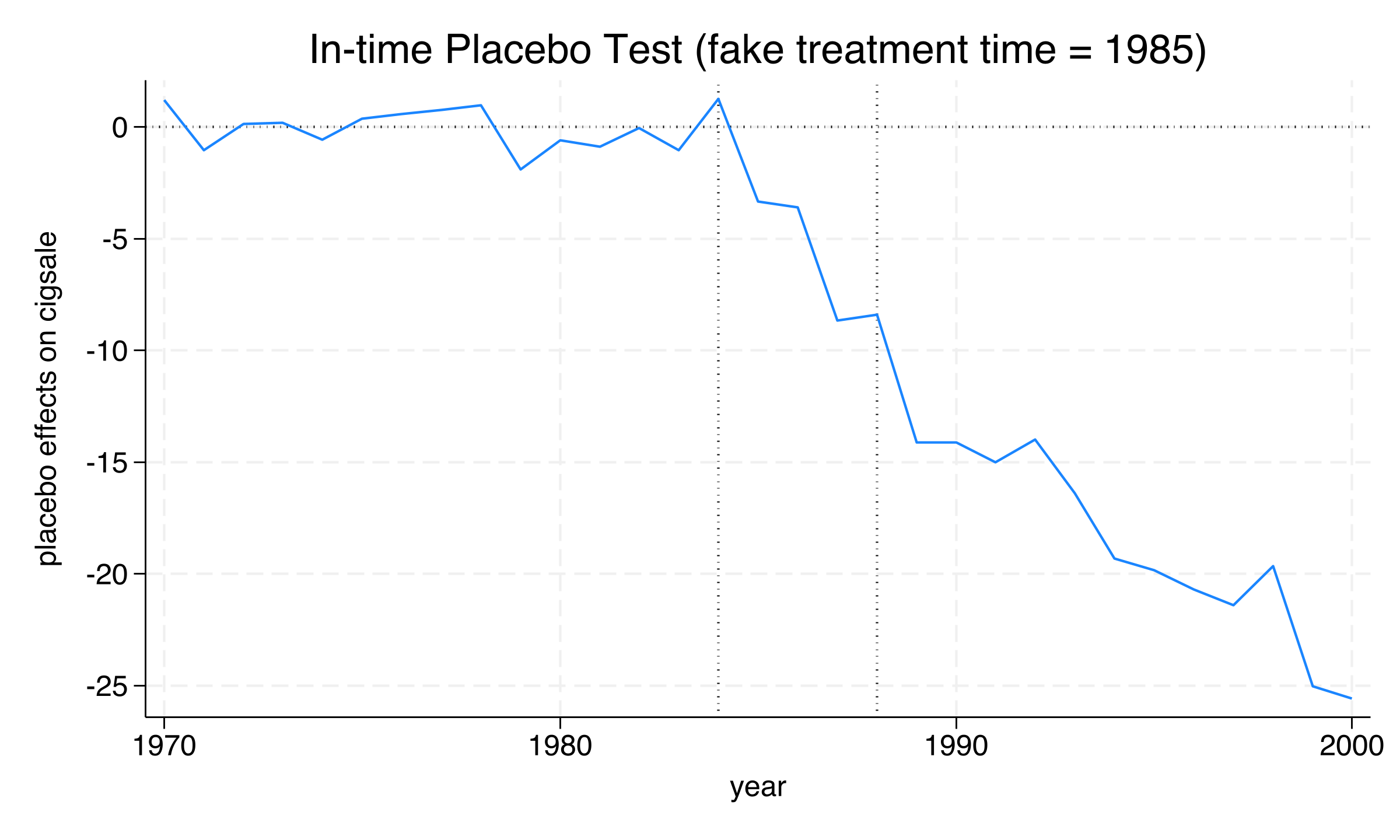
In-time placebo effect: smaller gaps during the fake 1985–1988 window, larger gaps after the real 1989 treatment.

Fake-period gaps average −5.99 packs. At the real date, the gap steps down by 5.74 packs, from −8.39 in 1988 to −14.12 in 1989, and it widens further in later years. The model thus finds much smaller effects at the fake date than after the real one. This pattern supports the design only in part, because the gap already steps down by a similar amount in 1987. The fake-period gaps are also not zero.

No single donor drives the sign of the effect: leave-one-out gaps stay negative

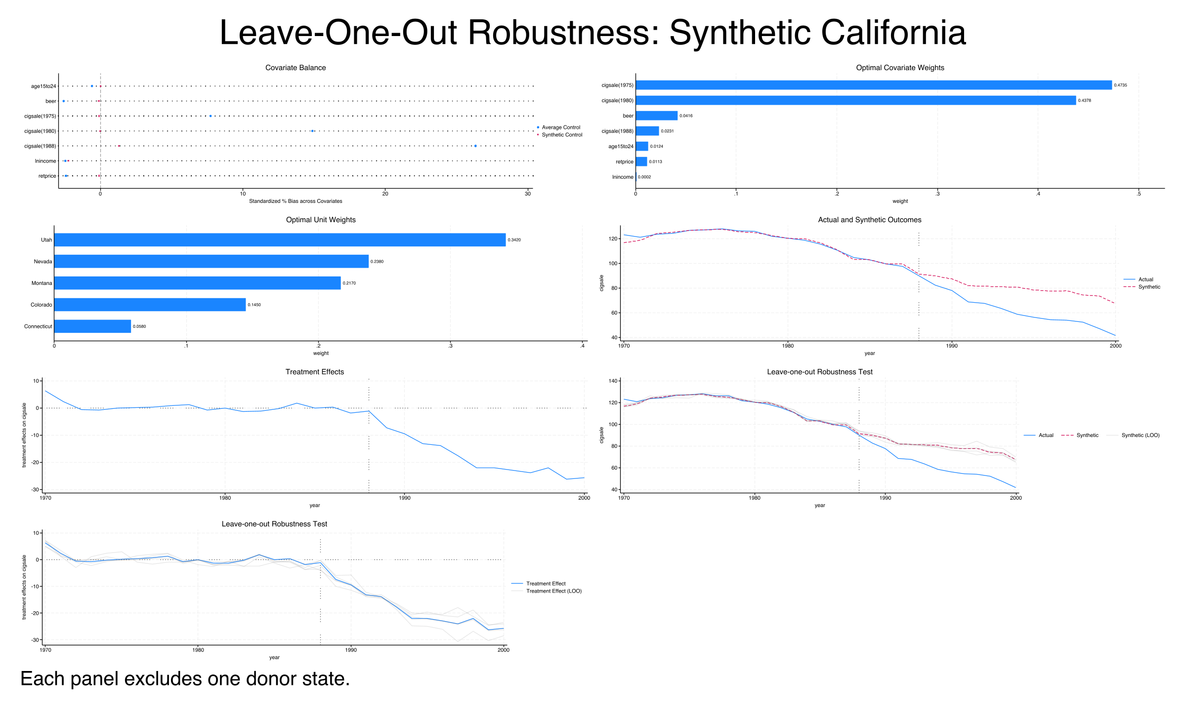
Leave-one-out output in seven panels. In the last two, each gray line drops one weighted donor, and the paths stay close to the full-pool fit.

We drop each of the five weighted donors in turn and refit the model. For 2000, the leave-one-out gaps range from −28.35 to −23.49 around −25.61, the value from the refit inside the same command. The spread of 4.87 packs is about 19% of the estimate. Every leave-one-out gap stays negative in every post-treatment year, even when Utah, with a third of the weight, is removed. The note printed under the figure is inaccurate: each gray line, not each panel, drops one donor. The deployed figure comes from the original run and still carries this note; the corrected do-file now writes an accurate one.

Does choosing controls by fit make this causal? Not by itself

Objection. A data-driven counterfactual is still a model. It cannot manufacture identification. Pre-1989 fit does not guarantee post-1989 validity.

Response. Correct. The ATT is credible only under no interference, no anticipation, no donor contamination, and good pre-treatment fit. SCM makes the last condition visible and disciplines the comparator. It cannot rule out cross-border shopping or an idiosyncratic donor such as Utah. It also gives no standard errors, so inference rests on the placebos.

We should take the critique seriously. The value of SCM lies in transparency; it does not deliver identification for free. The five-state synthetic control is sensitive to the predictor set: the ATT moves from −19.00 to −17.71 in the reduced specification of the in-time placebo, estimated with the real date. Utah, with its distinct smoking norms, shows how one idiosyncratic donor could matter. By design, the donor pool also excludes states with large tobacco control programs or large tax increases. Recent conformal-inference methods offer more formal confidence intervals.

Let the pre-treatment fit, not a parallel-trends assumption, earn the counterfactual.

This is the single takeaway of the talk. With one treated unit, a transparent weighted counterfactual that we can validate before treatment is more honest than an untestable parallel-trends story. For California, three checks support a negative effect: the placebo in space, the placebo in time, and leave-one-out. The in-time placebo, however, supports its timing only in part. Our estimate is that Proposition 99 cut sales by about 19 packs per capita per year over 1989–2000.