Causal Machine Learning and the Resource Curse

Who does mining help? Heterogeneous treatment effects with Stata 19

+0.149mining lifts nighttime lights

+0.405high-price premium · non-linear

96.90institutions moderate mining

Carlos Mendez

Nagoya University (GSID)

June 11, 2026

The Tension

Act I

One average effect hides who mining actually helps

The resource curse asks whether mineral wealth raises or wrecks development. Most studies answer with a single average effect.

But Hodler, Lechner & Raschky (2023) showed the answer bends with institutions. For whom does mining pay off — and where does it just bring conflict?

The central tension: a lone ATE is a press-release number. It says nothing about whether mining helps strongly-governed districts or weakly-governed ones. The resource-curse debate is really a debate about heterogeneity — institutional quality is the moderator. We need the CATE, not the ATE.

Stronger institutions, weaker mining benefit — the slope is the whole story

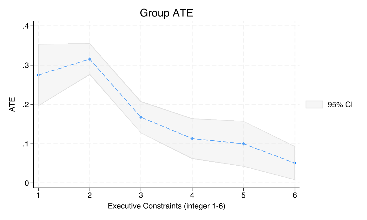
GATEs for the NTL mining effect (1-0) by executive constraints. Effect falls from 0.275 at the weakest constraints to 0.051 at the strongest.

Spoiler figure. Don’t read every bar yet — just plant that the mining effect is not one number. It marches downward as executive constraints rise: 0.275 at level 1, 0.051 at level 6. We earn this picture in Act II and return to it as the payoff in Act III.

Where we’re going

• The estimand: heterogeneous effects \(\tau(\mathbf{x})\), not one ATE
• A simulated resource-curse panel with known ground truth
• Stata 19’s cate: ATE, then GATEs, then per-district effects
• The lesson: institutions moderate mining, but not prices

The Investigation

Act II

The estimand is a function of \(\mathbf{x}\), not a single number

\[\tau(\mathbf{x}) = E\{Y_i(1) - Y_i(0) \mid \mathbf{X}_i = \mathbf{x}\}\]

The CATE is the average effect for districts with covariate profile \(\mathbf{x}\). Where \(\tau(\mathbf{x})\) bends, mining helps some districts more than others.

A single ATE is just \(E\{\tau(\mathbf{X})\}\) — this function averaged over everyone, discarding exactly the heterogeneity we want.

This is the formal move from ATE to CATE. Y(1) and Y(0) are potential outcomes — we see only one per unit. Identification rests on conditional independence given X (unconfoundedness): once we condition on the covariates, treatment is as-good-as-random. Stata’s cate estimates this whole function, then averages it to GATEs and the ATE.

A 3,000-row lab with ground-truth effects we can check against

• 300 districts × 10 years (2003–2012), 8 fictional countries
• Outcomes — log nighttime lights (development) and a conflict indicator
• Treatment — 4 levels: no mining (0), low / medium / high price (1/2/3)
• Moderators — executive constraints (1–6) and quality of government

Because the data-generating process is known, every estimate can be scored against its true value — a luxury real data never gives.

The treatment is highly imbalanced: 85% control, 5% in each treated price tier. This mirrors real mining data where few districts have active mines. The cate command handles it with honest random forests and sample-splitting. Ground-truth ATEs: 1-0 = 0.25, 3-1 = 0.30, 2-1 = 0.05.

A 4-level treatment becomes six binary CATE comparisons

Finding 1 — Mining effect

• 1 vs 0 · mining vs none
• 2 vs 0 · medium-price mining
• 3 vs 0 · high-price mining

Finding 2 — Price non-linearity

• 2 vs 1 · medium vs low (small)
• 3 vs 1 · high vs low (large)
• 3 vs 2 · high vs medium

Stata’s cate needs a binary treatment, so we subset to two groups at a time and run a generalized random forest on each contrast.

The six pairwise comparisons map directly onto the three paper findings. Mining-vs-none uses ~2,700 obs (well-identified); within-mining price contrasts use only ~300 obs (~150 per group), so expect wider CIs there.

Two estimators residualize the nuisance, then read off the signal

\[y = d\cdot\tau(\mathbf{x}) + g(\mathbf{x},\mathbf{w}) + \epsilon, \qquad d = f(\mathbf{x},\mathbf{w}) + u\]

PO (Partialing-Out)

• residualize \(y\) and \(d\) on \(\mathbf{x},\mathbf{w}\)
• regress residual on residual
• robust near propensity 0/1

AIPW (Augmented IPW)

• outcome model + propensity reweight
• doubly robust: one model can be wrong
• the conservative default here

g and f are nuisance functions — conditional means of outcome and treatment we estimate only to strip out predictable variation. Cross-fitting (xfolds 5) fits them on K-1 folds and scores the held-out fold, so no observation is scored by a model that saw it. PO and AIPW disagreeing is a diagnostic: overlap is suspect or a nuisance model is mis-specified.

Six lines estimate a heterogeneous mining effect in Stata 19

keep if treatment == 1 | treatment == 0
gen byte treat_1v0 = (treatment == 1)
global catevars exec_constraints quality_of_govt gdp_pc elevation /// moderators
cate aipw (ntl_log $catevars) (treat_1v0), ///
    controls(i.country_id i.year) ///
    rseed(12345) xfolds(5) omethod(rforest) tmethod(rforest)
categraph gateplot          // GATEs by subgroup
estat gatetest              // formal heterogeneity test

catevars (x) drive heterogeneity; controls (w) are country/year fixed effects for nuisance adjustment only. omethod/tmethod = rforest fits both nuisance models as random forests. The whole CATE suite — ATE, GATE, IATE, tests — comes from one command, no external packages. This is the load-bearing recipe the rest of the deck unpacks.

Raw means are biased: mining districts differ before any mine opens

Contrast	Naive diff	Ground truth
1 vs 0	0.109	0.25
3 vs 1	0.414	0.30
2 vs 1	0.099	0.05

Some confounders push the raw gap above the truth, some below — geography, institutions, and wealth all differ across mining status.

The naive difference-in-means mixes the causal effect with confounding. This is exactly what causal ML is for: adjust for the covariates flexibly and recover the true effect. The naive 1-vs-0 gap of 0.109 badly understates the 0.25 truth; cate will pull it back toward the right region.

With cross-fit AIPW, mining raises nighttime lights by 0.149

+0.149

AIPW ATE, mining vs none (SE 0.011, \(p<0.001\)); PO gives +0.194 on the same contrast

This is Finding 1, the headline policy number. Both estimators are positive and significant. PO (0.194) sits closer to the 0.25 ground truth; AIPW (0.149) is more conservative. The 0.045 gap between them is the model-disagreement diagnostic — here it just reflects finite-sample noise with 150 treated per tier. Mining also raises conflict: AIPW = 0.066, about 6.5 points above a 10.7% baseline.

Price effects don’t ramp — they jump only at the top

+0.405

High-vs-low price premium (AIPW 3-1, \(p<0.001\)); medium-vs-low is \(-0.011\), \(p=0.90\)

Finding 2: non-linearity. The step from low to medium prices does essentially nothing (−0.011, p = 0.90). The step from low to high prices does a lot (+0.405, p < 0.001). This is not a smooth dose-response — the price effect is dormant until prices spike. With only 300 obs the 3-1 estimate overshoots the 0.30 ground truth, but the qualitative jump is unmistakable.

A random forest chooses controls — it cannot relax identification

Objection. Machine-learning the nuisance functions can’t conjure a causal effect from observational data.

Response. Correct. \(\tau(\mathbf{x})\) is identified only under conditional independence given \(\mathbf{X}\) (unconfoundedness) and adequate overlap.

The forest estimates \(g\) and \(f\) — it cannot rule out an omitted confounder. The 3-vs-2 contrast even failed on overlap: a feature of honest estimation.

Steelman, don’t strawman. The forest just estimates the nuisance functions flexibly; identification still rests entirely on conditional independence and overlap. cate disciplines estimation; it does not deliver identification for free. The 3-2 price comparison has propensity scores near zero on 300 obs and AIPW refuses to report — the estimator telling you the data can’t answer the question. That honesty is exactly what you want.

The Resolution

Act III

Institutions moderate mining: the GATE test is decisive

96.90

\(\chi^2(5)\) for GATE equality by executive constraints (\(p<0.001\)) — effects are not homogeneous

This is Finding 3, the core result. estat gatetest rejects equal GATEs with chi2(5) = 96.90 across executive-constraint levels. The mining effect is systematically heterogeneous: 0.275 at the weakest constraints, 0.051 at the strongest — a 5x range. Note the sign flips relative to the paper (weaker institutions → larger effect here), but the structural finding — systematic moderation — replicates.

A second institutional measure tells the identical story

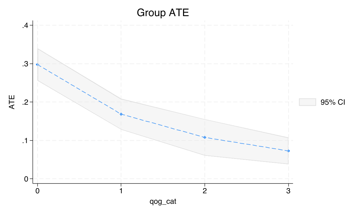
GATEs for the NTL mining effect (1-0) by quality-of-government quartiles: 0.298 in the lowest quartile, 0.073 in the highest. \(\chi^2(3)=69.19\), \(p<0.001\).

Robustness: swap executive constraints for quality of government and the downward slope survives — 0.298 in the bottom quartile, 0.073 in the top. Both institutional measures agree: weaker governance, larger mining effect. Two independent moderators pointing the same way is what makes the heterogeneity credible.

Subpopulation ATEs make the moderation concrete: 0.297 vs 0.092

Districts	ATE	SE	\(N\)
Weak institutions (exec \(\leq 2\))	0.297	0.022	558
Strong institutions (exec \(\geq 4\))	0.092	0.016	1,526

The mining effect is more than three times larger in weakly-governed districts — the same slope, now as a policy-ready contrast.

estat ate on subsets turns the GATE curve into two numbers a policymaker can act on. Mining buys far more nighttime light in weakly-governed districts (0.297) than in strongly-governed ones (0.092). This is the targeting payoff of CATE: it tells you where the treatment works hardest.

Prices behave oppositely — institutions do not bend the price premium

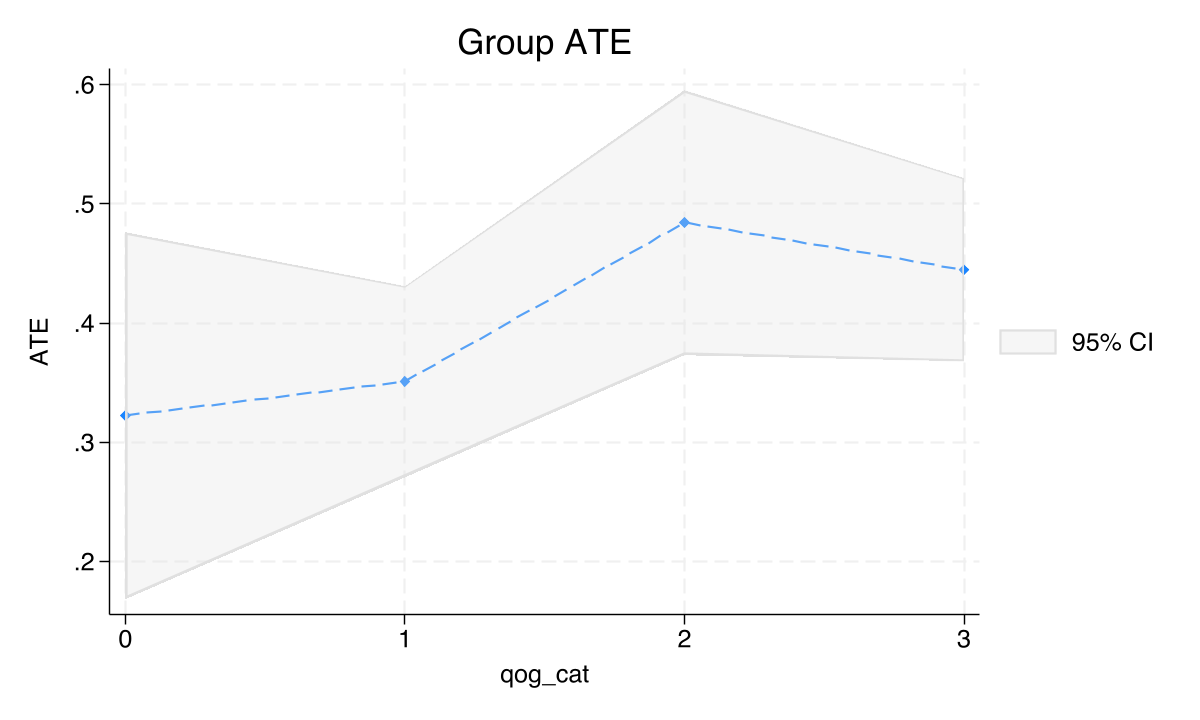
GATEs for the NTL price effect (3-1) by quality-of-government quartiles. No monotone slope; \(\chi^2(3)=5.81\), \(p=0.121\) — fails to reject equality.

The crucial asymmetry. For the price premium, the GATE test fails to reject equality (chi2(3) = 5.81, p = 0.121) — no systematic institutional moderation. Mining is local and institution-sensitive; global commodity-price shocks wash over districts regardless of governance. This is precisely the paper’s structural insight: institutions moderate mining, not prices.

And mining’s conflict effect is positive everywhere but flat across institutions

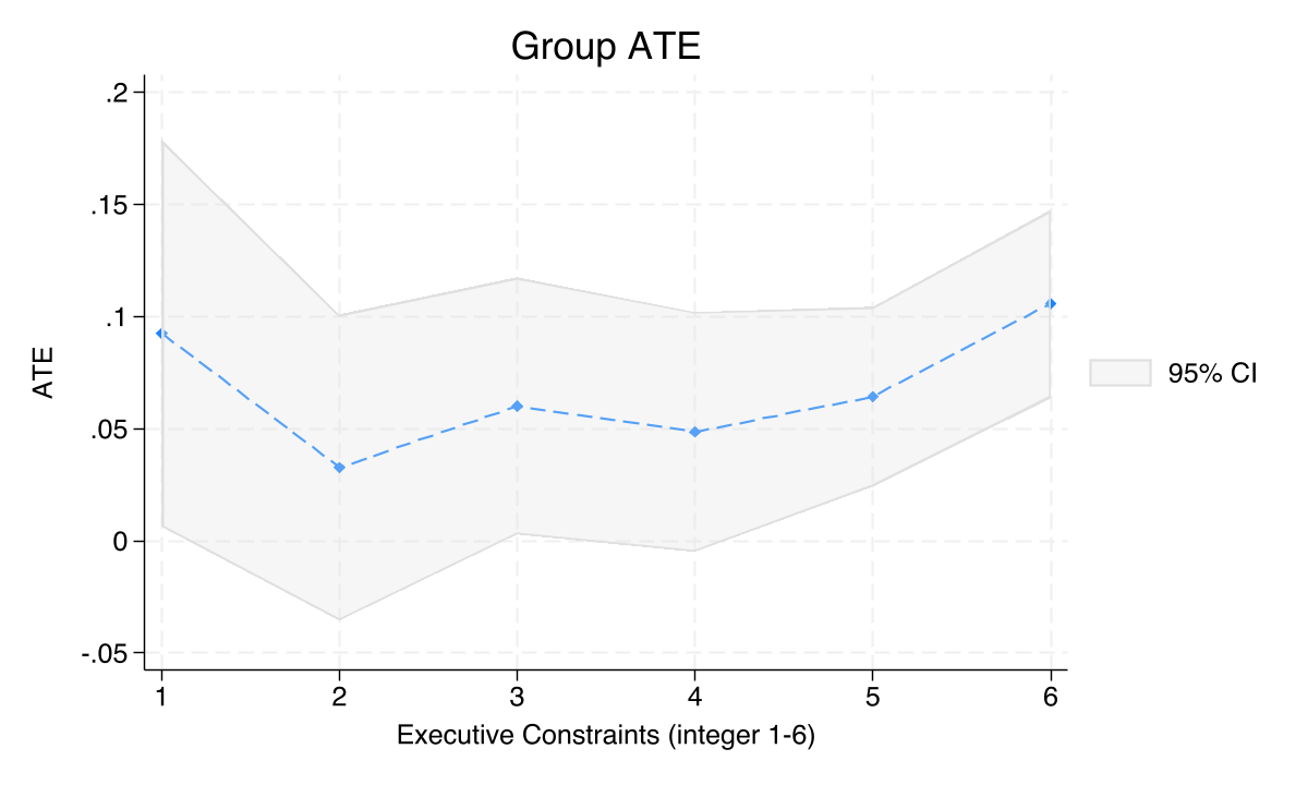
GATEs for the conflict mining effect (1-0) by executive constraints. All groups positive (0.033–0.106) but \(\chi^2(5)=5.00\), \(p=0.416\) — homogeneous.

Conflict rises with mining everywhere (every GATE positive), but the test fails to reject homogeneity (chi2(5) = 5.00, p = 0.416). So mining raises conflict broadly, without the institutional gradient that the development benefit shows. Heterogeneity is outcome-specific — you have to test it, not assume it.

Heterogeneity isn’t just group-level: every district gets its own effect

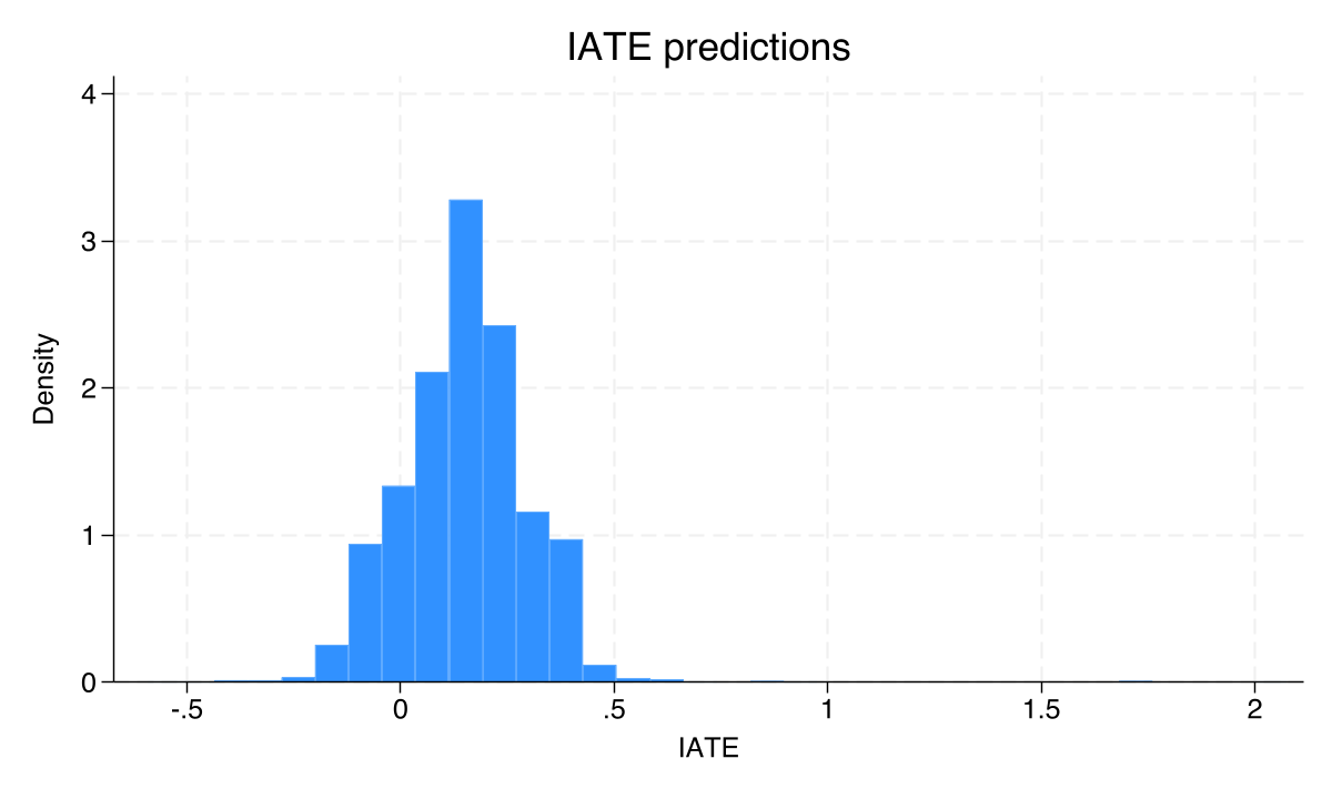
Distribution of individualized treatment effects \(\hat\tau(\mathbf{x}_i)\) for the NTL mining effect, centered near the 0.15 ATE with substantial spread. estat heterogeneity: \(\chi^2(1)=53.05\), \(p<0.001\).

IATEs are the finest grain: one effect per district. The spread of this histogram is the heterogeneity. The formal estat heterogeneity test (Chernozhukov et al.) rejects constant effects with chi2(1) = 53.05 — statistical license to read GATEs and IATEs rather than collapsing to an ATE.

The IATE function slopes down smoothly in institutional quality

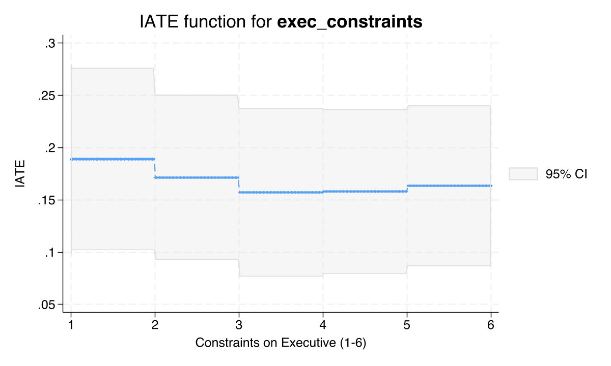
IATE function for the NTL mining effect as executive constraints rise, all other covariates at reference. The continuous downward trend confirms the GATE bars.

categraph iateplot holds everything fixed but one covariate and traces the IATE function. The downward slope in executive constraints is the continuous version of the GATE bar chart — same story, smoother view. quality_of_govt gives the same shape. A linear projection of the IATEs has R-squared only 0.024, because the forest captures nonlinearity a linear summary can’t.

Same data, same command, opposite conclusions about moderation

Mining effect

• GATE slope: steep, monotone
• \(\chi^2(5)=96.90\), \(p<0.001\)
• weak inst. 0.297 · strong 0.092

Price premium

• GATE slope: flat, noisy
• \(\chi^2(3)=5.81\), \(p=0.121\)
• no institutional gradient

The deck’s resolution in one frame. Both estimands come from the identical cate workflow on the identical panel — only the contrast and the moderator change. Mining is moderated; prices are not. The method didn’t impose this; the heterogeneity tests discovered it.

Test for heterogeneity — don’t average it away.

The single takeaway. A lone ATE would have told you “mining helps, prices help” and stopped. The CATE machinery in Stata 19’s cate — GATEs, subpopulation ATEs, IATEs, and formal tests — reveals that mining’s benefit depends on institutions while the price premium does not. That distinction is the policy-relevant finding, and you only see it if you let the data tell you where treatment effects vary.