Conditional Average Treatment Effects (CATE) with Stata 19

For whom does 401(k) eligibility build wealth?

$8,000doubly robust ATE

5.9×top-to-bottom effect ratio

$20,511GATE, top income group

Carlos Mendez

Nagoya University (GSID)

July 8, 2026

The Tension

Act I

“What is the effect?” is the wrong question — ask “for whom?”

The textbook workflow ends with one number: the Average Treatment Effect.

But no one acts on the average. The real question is who the program helps. That’s the CATE.

This is the central motivation. Policy makers, doctors, and managers never act on the average — they need to know who the program helps and who it leaves behind. A single ATE collapses a policy’s impact into one number, but the decision a policymaker faces is targeting: who should get the program. The whole deck is built to show that the average can hide an order-of-magnitude spread in effects.

The raw gap is $19,557 — but most of it is selection, not the program

Group	Mean assets	N
Eligible for 401(k)	$30,347	3,682
Not eligible	$10,790	6,231

Eligible workers are older, richer, more educated — so the $19,557 gap conflates the effect with who selects into eligibility.

This is the naive view, and it fails. If e401k were randomly assigned, $19,557 would be the ATE. It isn’t — eligibility is a function of which employer you chose. The job of every estimator that follows is to strip out the selection and recover the causal part.

Five income groups, one dataset — a fan from $1,400 to $20,511

GATE by income category with 95% bands: $4,087, $1,399, $5,154, $8,532, $20,511. The single average flattens all of this.

Spoiler figure. Don’t explain every bar yet — just plant that one policy produces wildly different effects across income groups, and that the top group gains roughly five times the average. We earn each piece in Act II and come back to this picture in Act III.

Where we’re going

• The estimand: \(\tau(x)\), the CATE — and what it takes to identify it
• The data: 9,913 households, eligibility vs net assets
• Stata 19’s cate — cross-fit lasso + a causal forest, in one command
• Heterogeneity: a test, a projection, GATE, GATES, a smooth gradient
• The lesson: the average household gains $8,000 — but a quarter gain nothing

The Investigation

Act II

The estimand is a function, not a number: \(\tau(\mathbf{x})=E[y(1)-y(0)\mid \mathbf{x}]\)

\[\tau(\mathbf{x}) = E\big[\,y(1) - y(0) \mid \mathbf{x}\,\big]\]

The average effect among households whose covariates equal \(\mathbf{x}\). Where \(\tau(\mathbf{x})\) bends with \(\mathbf{x}\), the program helps some households more than others.

The single ATE is just \(E[\tau(\mathbf{X})]\) — the CATE averaged over the population.

The CATE is a function of x, not a scalar. If τ(x) were constant we’d be back at the ATE. The whole point of the deck is that it is NOT constant. Note y(1) and y(0) are potential outcomes — we only ever observe one per household, so this is fundamentally a missing-data problem.

Two assumptions do the causal work — the forest only fits the function

Unconfoundedness

\[y(1),y(0) \perp d \mid \mathbf{x}\]

• No unmeasured confounders given the covariates
• Justified here by a rich demographic vector

Overlap

\[0 < \Pr(d=1\mid \mathbf{x}) < 1\]

• Every profile could be treated or not
• 37% / 63% split → comfortable overlap

Machine learning chooses controls flexibly; it cannot manufacture identification.

This is the load-bearing slide for rigor. The causal forest gives us a flexible τ̂(x), but identification rests entirely on these two assumptions — they are assumptions about the world, not about the estimator. Overlap is what keeps the inverse-propensity weights in AIPW from blowing up.

The lab: 9,913 households, eligibility → net financial assets

• Outcome — net total financial assets ($), wildly right-skewed: mean $18,054, median just $1,499
• Treatment — employer-offered 401(k) eligibility (not participation): 37.1% eligible
• Covariates — age, education, income, pension, marriage, two-earner, IRA, homeownership

assets3, the canonical Chernozhukov–Hansen excerpt shipped with Stata 19.

The heavy right tail of assets is exactly why a single-number ATE struggles — skewness 10.6, kurtosis 187. When the outcome is that skewed, the effect is almost guaranteed to be heterogeneous across the income distribution.

cate runs cross-fit lasso and a causal forest in one command

webuse assets3, clear
* covariates driving the heterogeneity = nuisance controls here
global catecovars age educ i.incomecat i.pension i.married i.twoearn i.ira i.ownhome

cate po (asset $catecovars) (e401k), rseed(12345671)

Lasso for the nuisance functions (cross-fitted), a generalized random forest for \(\tau(\mathbf{x})\), honest-tree bootstrap for the CIs — Stata 18 needed hand-rolled loops.

The full do-file is in the post; these are the load-bearing lines. cate po is the partialing-out estimator: it residualizes both the outcome and the treatment against the covariates (cross-fitting), then fits a causal forest on the residuals. rseed makes the cross-fitting reproducible.

Two routes to the same object: PO is robust, AIPW is efficient

PO (partial-linear)

• Residualize \(y\) and \(d\) on \(\mathbf{x}\), then regress
• Transparent; robust when propensities near 0 or 1
• ATE \(= \$7{,}937\)

AIPW (interactive)

• Separate outcome models + propensity reweight
• Doubly robust: only one nuisance model need be right
• ATE \(= \$8{,}120\)

Both return a per-household effect function \(\hat\tau(\mathbf{x}_i)\) — they differ only in how they map nuisances into it.

PO and AIPW make different model assumptions but produce the same kind of object. AIPW’s double robustness is the headline property: it stays consistent if EITHER the outcome model OR the propensity model is correct. The cost is sensitivity to extreme propensities, which is why overlap matters.

Three estimators bracket the ATE within a $183 spread

$8,000

Parametric AIPW $8,019 · ML PO $7,937 · ML AIPW $8,120 — agreement across very different specifications

When a mature parametric estimator and two machine-learning estimators that share nothing under the hood all land within $183, you can report the average with high confidence. This is the deck’s central robustness check. Now the real question: what does that $8,000 average hide?

First, does the effect vary at all? The test says yes

Estimator	\(\chi^2(1)\)	\(p\)	Verdict
cate po	4.11	0.043	reject homogeneity
cate aipw	5.54	0.019	reject homogeneity

estat heterogeneity — \(H_0:\ \tau(\mathbf{x})\) is constant. Both reject at 5%, so the heterogeneity hunt is not chasing noise.

Before exploring HOW the effect varies, we ask WHETHER it varies. Both estimators reject the constant-effect null. AIPW rejects more strongly (p = 0.019 vs 0.043), consistent with its higher efficiency when both nuisance models are well-specified. This licenses everything that follows.

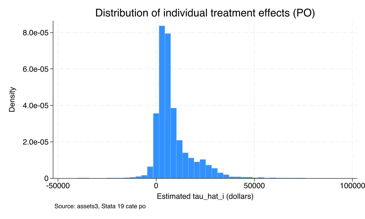
The average of $7,937 hides a long right tail of large effects

PO-estimated individual effects \(\hat\tau_i\) across 9,913 households: a tight mode near $5–10k, a tail past $80k, and a small mass near or below zero.

This is the visual answer to “is the average hiding something?” The mean of $7,937 sits close to the median, but the spread is enormous. Most households cluster around a modest positive effect; a long right tail extends past $80,000; a small left tail dips negative. The next views describe WHO sits in that right tail.

A linear projection of \(\hat\tau_i\) says income is the only strong signal

Covariate	Effect on \(\hat\tau_i\) ($)	\(p\)
Highest income category	+18,195	0.001
Homeowner	+3,163	0.058
Age (per year)	+205	0.082
Education (per year)	−442	0.365

estat projection: the only coefficient significant at 1% is the top income category. \(R^2=0.0045\) — most heterogeneity is nonlinear, captured by the forest, not the projection.

A causal forest fits τ̂(x) flexibly but a flexible function is hard to summarize. The linear projection answers “which variables shift the predicted effect?” Income dominates. The low R² is a feature, not a bug — it tells us the real structure is curvature the projection can’t see, which is exactly why we need GATE and the series fit.

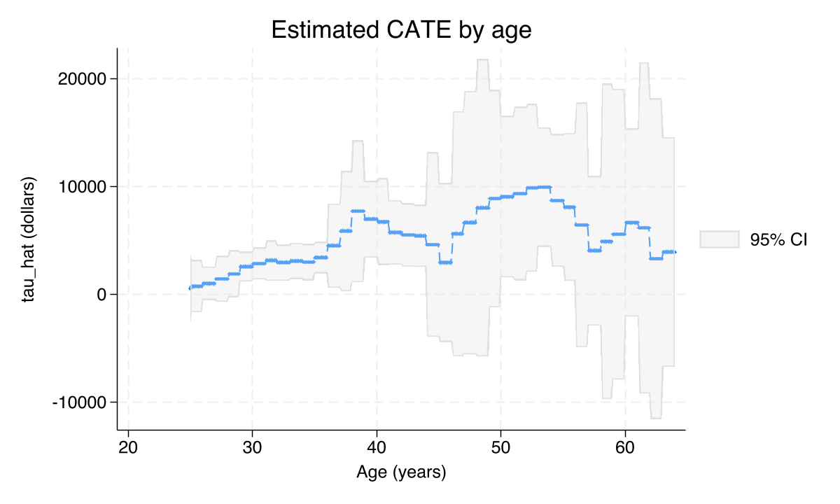
Effects climb with age; education barely moves them

PO-estimated CATE by age (others fixed at means): slightly negative in the mid-20s, clearly positive by 35–40, still rising through the 50s.

categraph iateplot holds every covariate but one at reference values and varies the one of interest — a slice through the multidimensional CATE surface. 401(k) eligibility is most valuable to workers with the financial slack and planning horizon to use tax-deferred saving. Bands narrow where the data is dense and widen at the extremes.

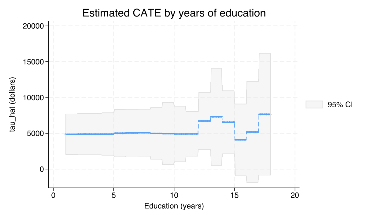
Education is a flat line — once you know income, it adds nothing

PO-estimated CATE by years of education: broadly flat around $1–3k from 8 to 18 years of schooling.

A useful negative finding, and it matches the projection (the education coefficient was small and not significant). Conditional on income, education carries almost no extra information about who benefits. Negative findings discipline the story: not every plausible moderator matters.

Let the data sort the households: the top quartile gains 5.9× the bottom

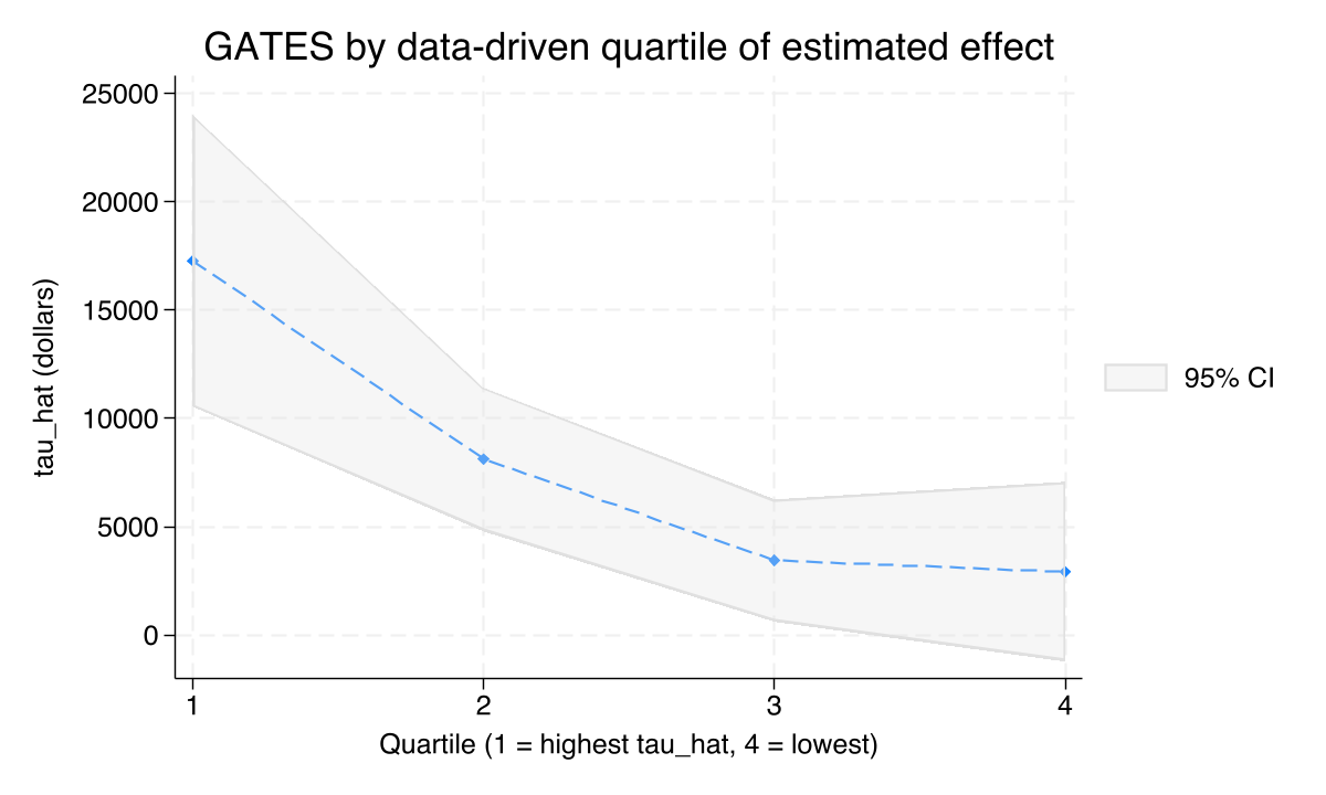
GATES by data-driven quartile of predicted effect: $17,279 → $8,121 → $3,444 → $2,919. A clean monotonic ladder; the bottom bin is not distinguishable from zero.

GATES flips GATE around: instead of naming groups in advance, it sorts households by their predicted effect, bins into quartiles, and reports the actual response in each. Cross-fitting protects against p-hacking — each unit’s bin comes from an out-of-sample prediction, so it can’t leak its own outcome. The 5.9× ratio is the single most informative summary of heterogeneity here.

The high-effect quartile earns $35,878 more than the low-effect one

Covariate	Top quartile	Bottom quartile	Diff	\(t\)
Income ($)	62,739	26,861	35,878	56.2
Age (years)	45.2	35.0	10.2	35.7
Education (years)	14.0	12.7	1.4	18.6

estat classification: the data sorted itself; income is the dominant marker of who responds. All three gaps have \(t>18\).

The data did the sorting; now we ask what makes the top quartile different. The high-effect group is older, richer, and more educated — but income is the dominant signal, fully consistent with the projection and the GATE-by-income picture. The story: 401(k) eligibility helps people who already had latent demand for retirement saving and the slack to act on it.

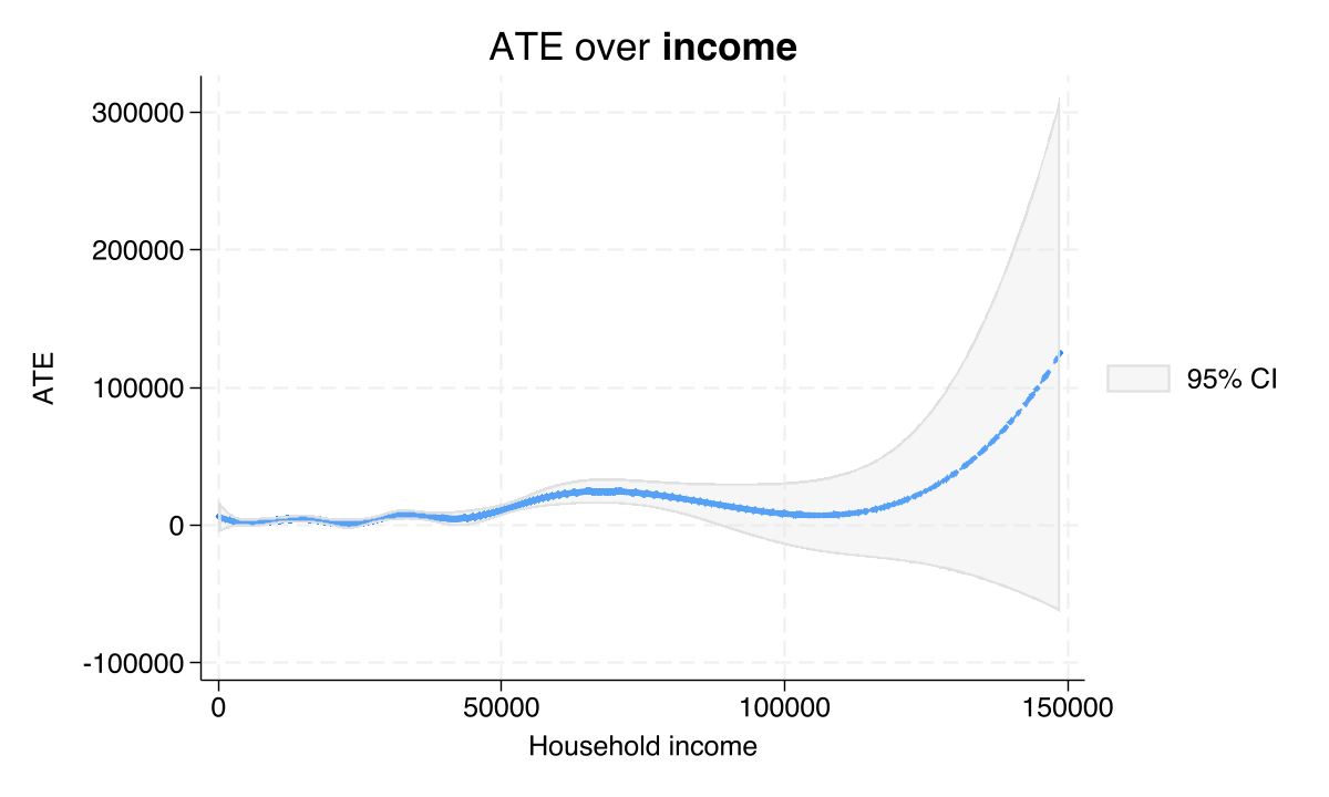
A smooth fit: each extra $1,000 of income adds ~$213 to the effect

Cubic B-spline of \(\hat\tau\) vs household income (income \(\le\) $150k): a smooth upward slope, steepest in the middle of the distribution.

estat series marginalizes over the other covariates and fits a flexible smoother against income — the cleanest dose-response view. The reported “Effect” is an average derivative: 0.213 (SE 0.050, p < 0.001). In dollars, each extra $1,000 of income raises the predicted treatment effect by about $213. The slope is not constant, which is why a single linear coefficient only partly captured the gradient.

The Resolution

Act III

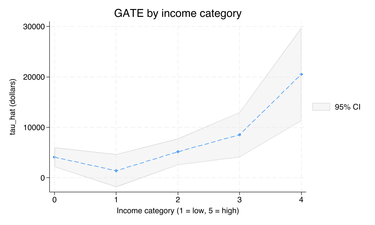
The top income group gains $20,511 — five times the average household

$20,511

GATE, highest income category (vs ~$4,000 at the bottom). Joint test of equality across groups: \(\chi^2(4)=18.44\), \(p=0.001\)

Back to the Act-I spoiler, now earned. Five GATEs span an order of magnitude — $4,087, $1,399, $5,154, $8,532, $20,511 — and the joint test rejects equality at p = 0.001. The marginal household at the top gains about $20,500; the marginal household at the bottom gains about $4,000; the middle-low group (category 1) gains effectively nothing. A blanket program ignoring this would badly misjudge the targeting.

A quarter of households gain little or nothing — invisible in the ATE

The bottom GATES quartile is $2,919 with \(p=0.167\) — not statistically distinguishable from zero.

Combined with the small negative left tail of the histogram: roughly one in four households appears to gain close to nothing from eligibility.

This is the nuance the headline $8,000 erases entirely. About a quarter of the sample receives close to zero — or even slightly negative — net benefit. A policy designed off the average alone would assume everyone gains $8,000, which is simply false for the bottom quartile.

Does the causal forest make this causal? No — the assumptions still carry it

Objection. A machine that flexibly selects controls surely earns us the causal interpretation.

Response. It does not. \(\tau(\mathbf{x})\) is identified only under unconfoundedness and overlap. The forest fits the function; it cannot rule out an unmeasured confounder.

Steelman, don’t strawman. The cate command disciplines estimation; it does not relax the identifying assumptions. If, say, employer match rates vary with income and we never observe them, the income gradient is biased. The most credible threat here is an income-correlated unobserved confounder like the employer match rate. Honest practice: report the gradient as conditional on the unconfoundedness assumption, and flag the overlap check (teffects overlap / estat osample) as the natural follow-up.

The average is a press release; the CATE is the policy

• ATE \(\approx \$8{,}000\) — agreed across three estimators within $183
• But effects span $1,400 → $20,511 across income groups (\(p=0.001\))
• Income is the moderator: +$213 per $1,000, +$18,195 at the top
• One in four households gains essentially nothing

The full summary in four lines. Each is anchored by a number from the post. The takeaway for design: a 401(k) eligibility expansion delivers far larger asset gains to high earners than to low earners — though the lowest-income households still gain a real, significant ~$4,000.

Estimate the CATE, not just the ATE — the average is hiding who your policy actually helps.

The single sentence to remember, and the resolution of the Act-I hook. The same data, the same program — yet the answer to “does it work?” depends entirely on “for whom?” Stata 19’s cate command makes that question a one-command workflow.