From DiD to SDID

A ladder of synthetic control estimators, and what Brexit cost the UK

2.76%UK GDP shortfall at end-2018 · SDID

96%of the time weight on one quarter

23donor countries in synthetic Britain

Carlos Mendez

Nagoya University (GSID)

August 4, 2026

The Problem

Act I

There is only one United Kingdom, and it voted to leave

On 23 June 2016 the UK voted to leave the European Union.

To price that decision we need the UK that stayed. It does not exist in any dataset.

Where do we get the counterfactual?

No country is a twin of the UK, so the comparison has to be built, not picked.

The fundamental problem of causal inference with a single treated unit. No country is a perfect twin of the UK, so we cannot pick a comparison — we have to build one.

Build it out of the countries we do observe

24 OECD economies, quarterly log real GDP, 1995Q1 to 2020Q4.

• 1 treated unit: the United Kingdom
• 23 donors, from Australia to the United States
• 86 pre-treatment quarters to fit against
• 2 evaluation dates: 2018Q4 and 2019Q4

Weight the donors. Match the UK for twenty-one years. Read the gap.

Eighty-six quarters of tracking are what license reading the post-2016 gap as an effect.

Give each donor a weight, require the blend to track the real UK quarter by quarter through the two decades before the referendum, and whatever gap opens after 2016 is the estimate.

One line in a crowd

Log real GDP for 24 OECD countries, 1995–2020: the UK in orange among 23 grey donor paths, dashed line at the 2016 referendum.

No single donor tracks the UK — which is exactly why we blend them rather than pick one.

No single donor tracks the UK — which is why we blend them rather than pick one. But notice 2008-09: every line collapses together. That synchronised movement is a common factor, and it is what the demeaned and time-weighted stages are built to exploit.

The previously published answer was 2.4%

Born et al. (2019): the referendum cost the UK 2.4% of GDP by end-2018.

That number came from one estimator with one set of choices.

This deck climbs the whole ladder and asks whether 2.4% survives.

2.4% is one estimator’s answer, not the dataset’s answer.

The full citation is Born, Müller, Schularick and Sedláček (2019), using this same OECD panel. Their specification matches on six covariates — which, as we will see in the verdict, is the single choice that separates their number from everything on this ladder.

The Ladder

Act II

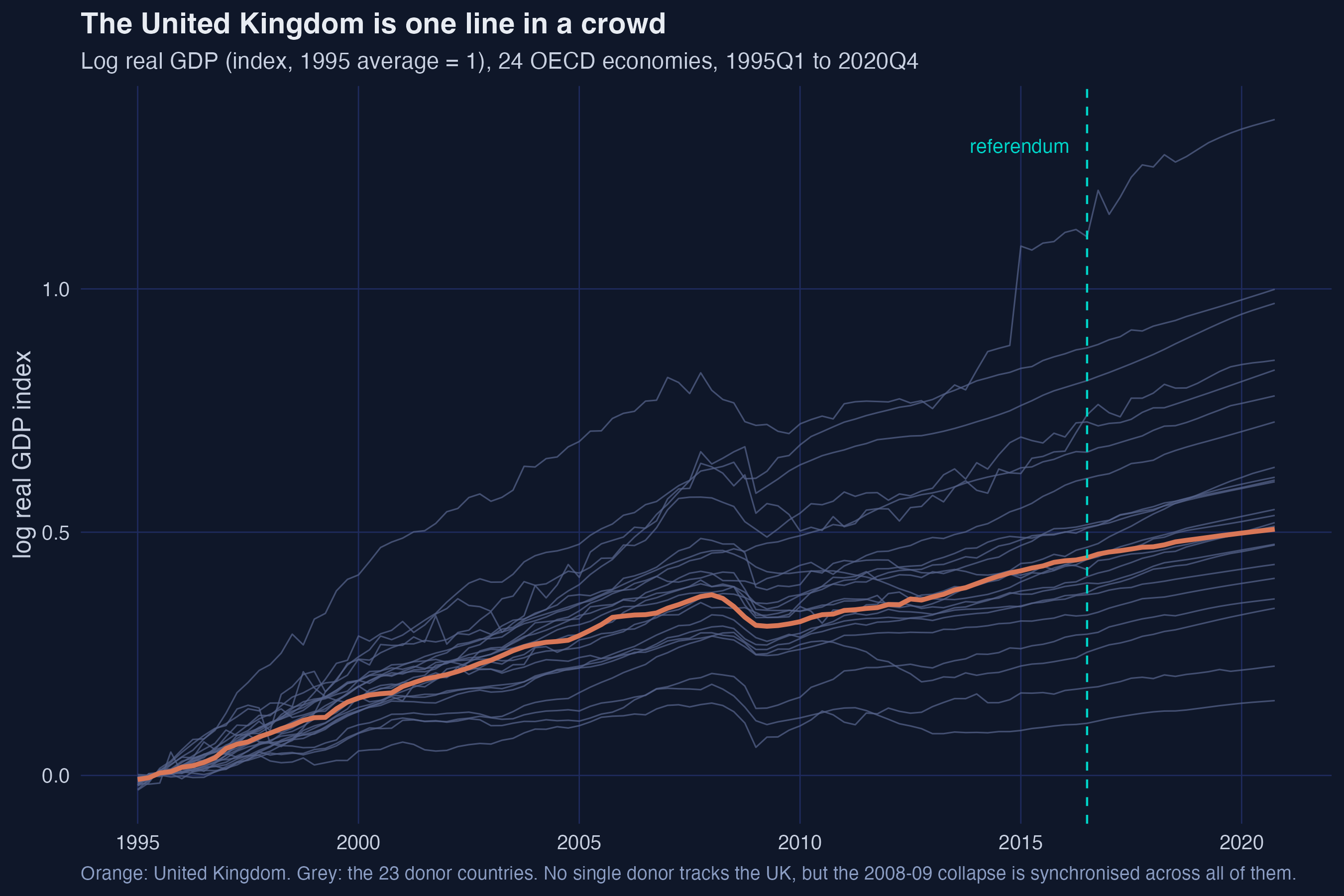
Every estimator is the same regression

\[\left(\hat{\tau}, \hat{\alpha}, \hat{\beta}\right) = \arg\min \sum_{j} \sum_{t} \left( y_{j,t} - \alpha_j - \beta_t - w_{j,t}\tau \right)^{2} \hat{\omega}_j \hat{\lambda}_t\]

Outcome on a country effect, a quarter effect and a treatment dummy — weighted by \(\hat{\omega}_j\) and \(\hat{\lambda}_t\).

Every stage that follows is a choice of which weights to fix and which to estimate.

This is the only equation in the deck worth memorising. Everything that follows is a choice of which weights to fix and which to estimate.

Four settings of the same dials

Stage	\(\omega\)	\(\lambda\)	unit effect
DiD	fixed \(1/J\)	fixed	yes
SC	optimised	none	no
DSC	demeaned	fixed	yes
SDID	demeaned	optimised	yes

Two banks of faders. DiD leaves both flat, SC moves one, SDID moves both.

Turning \(\lambda\) on is the only thing that separates DSC from SDID.

One solver, used five times

simplex_ls <- function(A, b, ridge = 1e-10) {
  k <- ncol(A)
  w <- solve.QP(Dmat = crossprod(A) + ridge * diag(k),
                dvec = crossprod(A, b),
                Amat = cbind(rep(1, k), diag(k)),   # sum(w) = 1; w >= 0
                bvec = c(1, rep(0, k)),
                meq  = 1)$solution
  w[w < 1e-10] <- 0
  w / sum(w)
}

Hand it the donors’ pre-treatment paths and it returns \(\omega\). Hand it the transpose and it returns \(\lambda\).

One quadratic program does five jobs: \(\omega\), demeaned \(\omega\), \(\lambda\), and both halves of MASC’s cross-validation.

Minimise a sum of squares over the simplex — non-negative shares that add to one. The 1e-10 on the diagonal is numerical hygiene so the Cholesky factorisation never fails; it is not the regularisation parameter of Arkhangelsky and coauthors.

Stage 0 — the ground floor: every donor counts the same

w_did <- rep(1/23, 23)
b_did <- mean(Z1 - Z0 %*% w_did)

4.98% at 2018Q4 — nearly double everything else.

Its pre-treatment fit error is 0.0218, four times synthetic control’s.

DiD answers loudest and fits worst — which is the whole reason the ladder has more rungs.

The post numbers these estimators 1 through 6; the deck calls DiD Stage 0, the ground floor, because it turns none of the dials. Throughout, \(T_0\) = 86 is the number of pre-treatment quarters, the synthdid convention; the papers write the same quantity as \(T_0 - 1\).

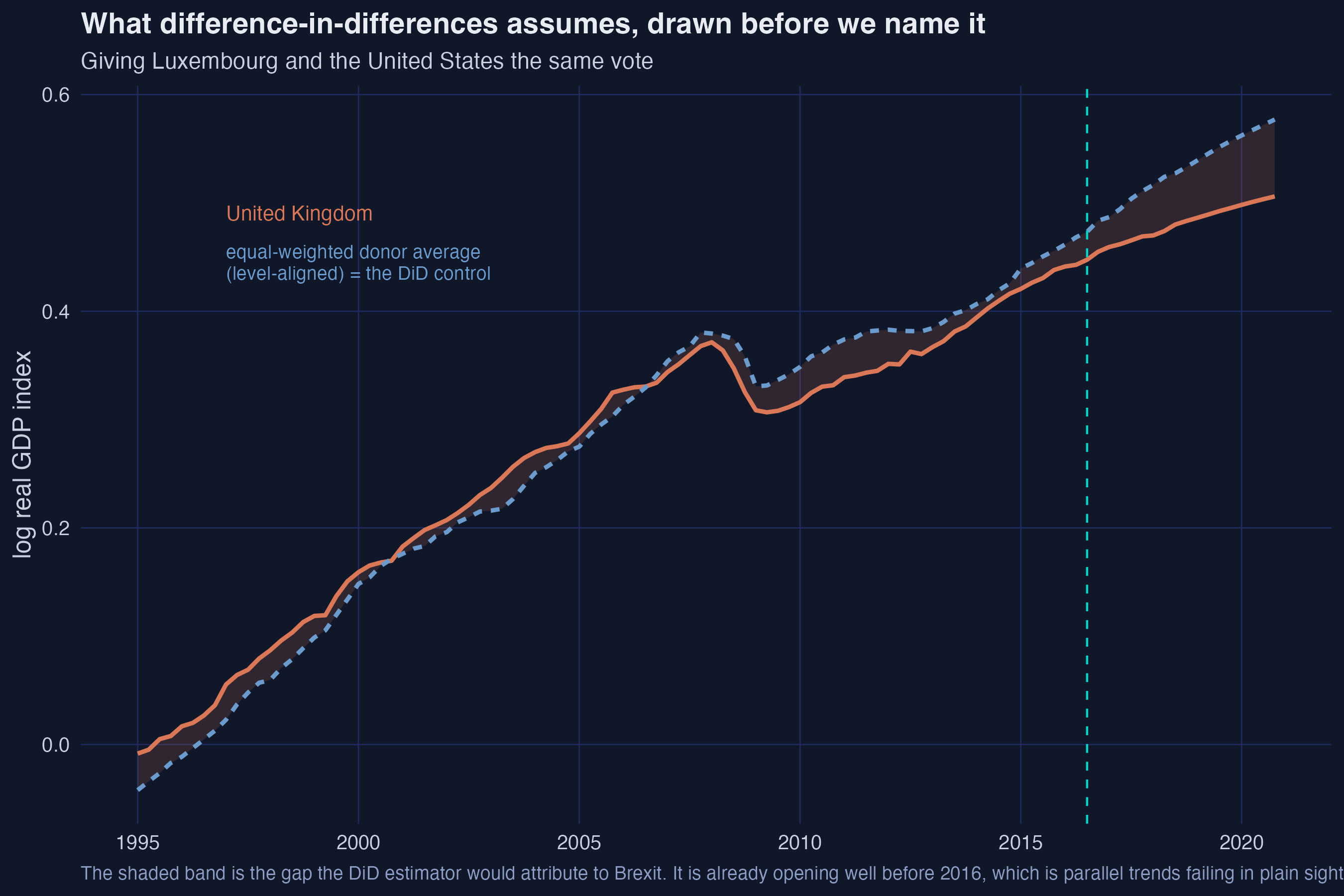
Parallel trends, failing in plain sight

The UK against the level-aligned equal-weighted average of the 23 donors, with the growing gap shaded in orange.

DiD is fitting a divergence that began in 2013 and calling it Brexit.

Stage 1 — letting the data pick the weights cuts the fit error four-fold

\[\hat{\omega}^{sc} = \arg\min_{\omega \in \mathbb{W}} \sum_{t=1}^{T_0} \Big( y_{1,t} - \sum_j \omega_j y_{j,t} \Big)^{2}\]

Here \(T_0 = 86\), the number of pre-referendum quarters (the synthdid convention); the papers write the same sum as running to \(T_0-1\).

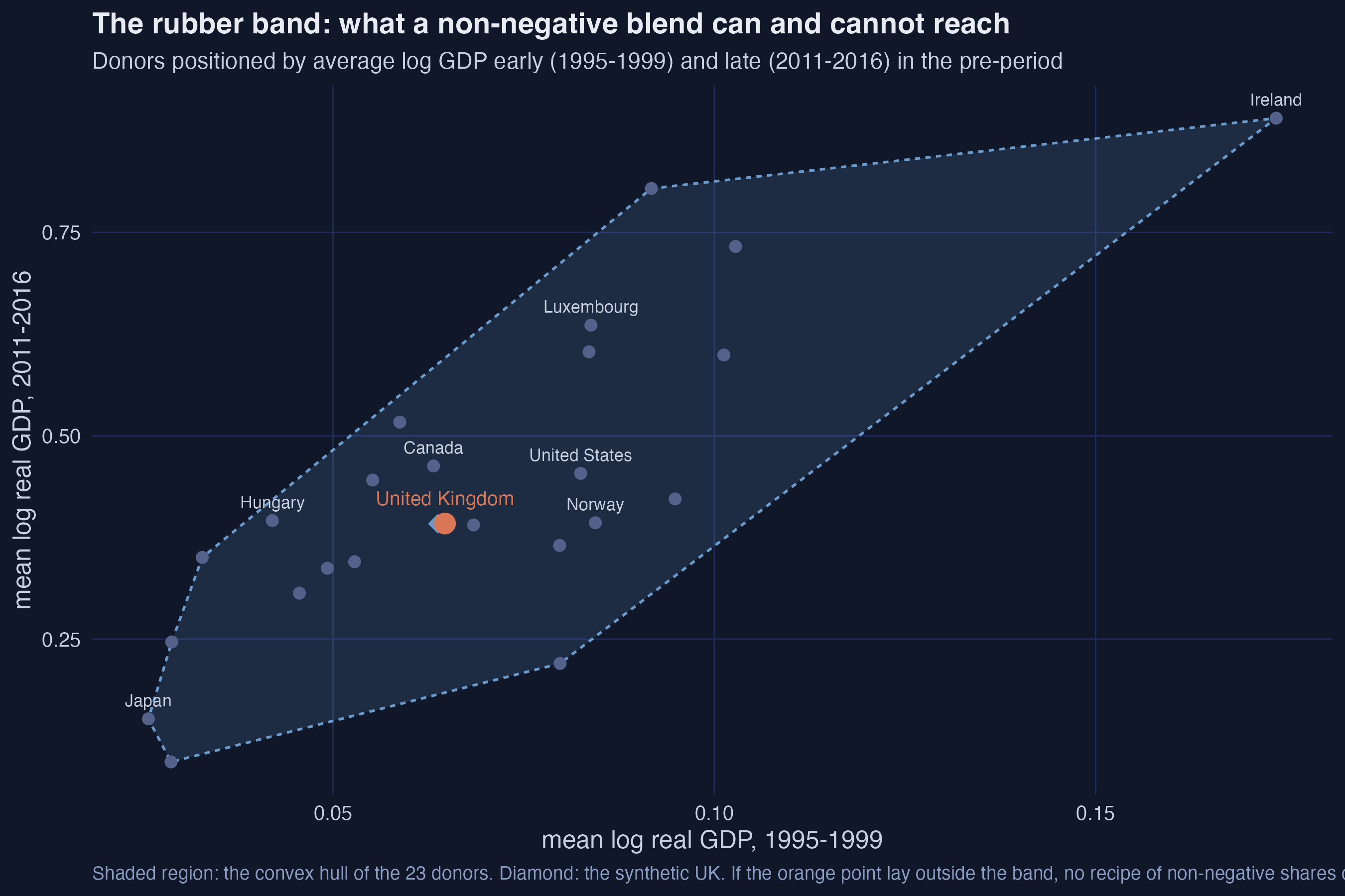
Weights that are non-negative and sum to one: the blend must stay inside the donors’ convex hull.

Synthetic Britain is roughly one-fifth Hungary, one-fifth the US, one-fifth Japan, one-sixth Canada.

3.06% at 2018Q4. Pre-treatment fit error 0.0057.

0.0057 against DiD’s 0.0218 — a quarter of the error, and the entire argument for the method.

Everything inside the rubber band is reachable; nothing outside it is

Donors plotted by average log GDP early and late in the pre-treatment window, with the convex hull shaded and the UK inside it.

The UK sits comfortably inside the hull, which is why synthetic control works well here.

Pins on a corkboard, a rubber band snapped around them. Everything inside is reachable by a non-negative blend; nothing outside is. If the UK’s pin fell outside, you would need a negative amount of some country.

Stage 2 — Demeaned SC: allow a level gap

SC has no intercept, so it rejects a blend that moves in perfect parallel but sits slightly below.

Demean first, then add the average pre-treatment gap back as a constant.

\[b^{dsc} = \frac{1}{T_0} \sum_{t} \Big( y_{1,t} - \sum_j \hat{\omega}_j y_{j,t} \Big)\]

The average gap over the 86 pre-referendum quarters — the same \(T_0\) convention as above.

Adding \(b^{dsc}\) is algebraically identical to switching the unit fixed effect back on.

The offset is tiny, and that is the finding

Here \(b^{dsc} = +0.0024\) — a quarter of one percent. The estimate moves 3.06% → 2.99%.

A small adjustment means the SC fit was already level-balanced. On a dataset where the treated unit sits awkwardly, this term does real work.

The anticlimax is the result: there was almost no level gap to correct.

Stage 3 — SDID: choose which quarters to trust

DSC averages all 86 pre-treatment quarters equally. 1995 gets as much say as 2016.

The time-weight problem is the unit-weight problem, transposed.

• \(\omega\): which countries, blended, reproduce the UK?
• \(\lambda\): which quarters, blended, reproduce the treatment quarter?

Same solver, transposed argument, and the cross-sectional mean removed instead of the time-series mean.

\(\lambda\) is \(\omega\)’s problem run on the transpose — one solver, two directions.

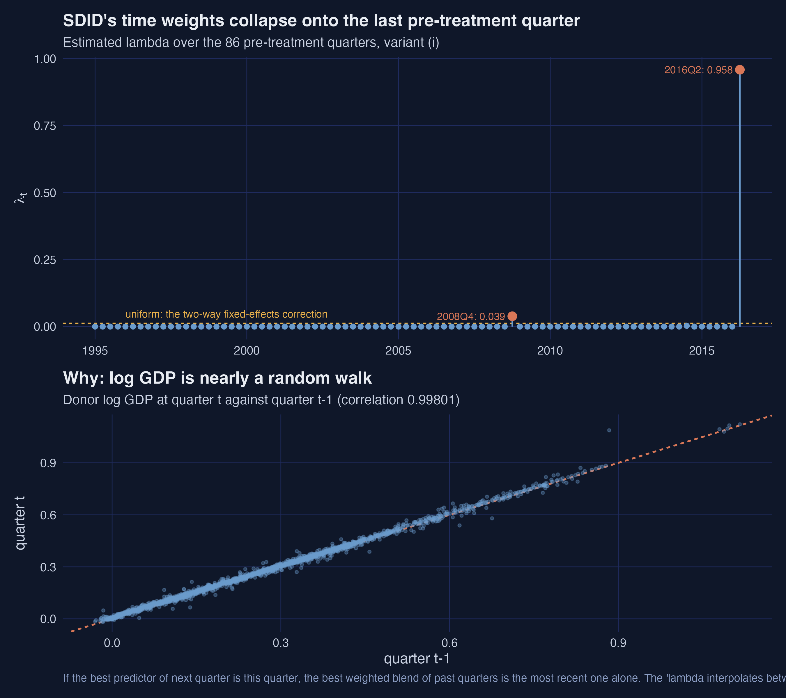
And the time weights collapse

The estimated time weights as a stem plot, and donor log GDP at quarter \(t\) against \(t-1\) lying almost on the 45-degree line.

96% of the weight lands on a single quarter, 2016Q2.

Log GDP is nearly a random walk, so the best blend of past quarters is the most recent one alone. 2.76%.

The collapse is a property of the data, not a bug in the code.

The Pivot

Act III

Two ways to be wrong

For any weighted counterfactual, the bias splits exactly in two:

\[\text{Bias} = \underbrace{B^{ext}}_{\text{wrong place}} + \underbrace{B^{int}}_{\text{curved function}}\]

Extrapolation bias — the blend’s characteristics do not match the treated unit’s.

Interpolation bias — the blend matches, but the outcome curve bends.

The average of outcomes is not the outcome at the average.

Neither name means what you would guess.

Because the two pieces add up exactly, any estimator can be asked which half it attacks.

A 3.4 kg bird, and two ways to get the roasting time wrong

A 3.4 kg bird. The chart lists 3 kg and 4 kg.

Extrapolation bias: you look up 5 kg. Wrong row.

Interpolation bias: you average the two rows. Right rows, curved chart.

Fixing one does nothing for the other.

Roasting time bends with weight, so the average of the 3 kg and 4 kg times is not the time for a 3.4 kg bird. The two errors are independent — that is the whole point of the decomposition.

Only one row is dark in both columns

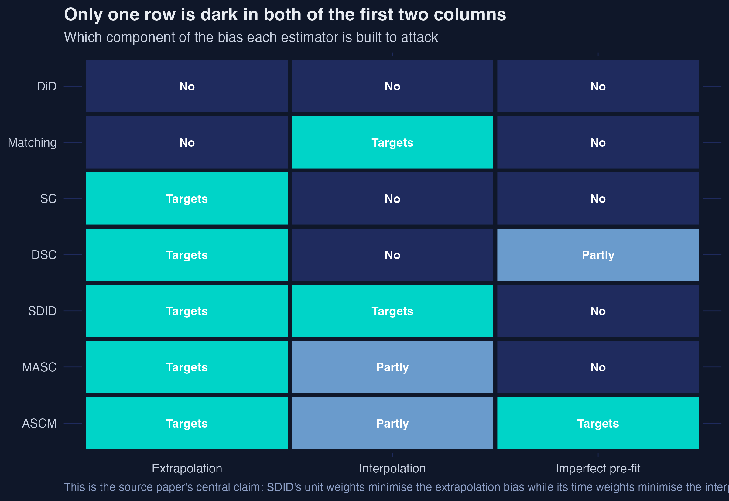
Estimators as rows, bias types as columns: only the SDID row is dark in both the extrapolation and interpolation columns.

SC’s unit weights kill extrapolation bias. Matching kills interpolation bias.

SDID’s time weights are what let one estimator target both.

The counterweight the source paper supplies itself, and it belongs in the spoken version: SDID “targets” both biases, but it pays for the privilege by estimating 85 extra parameters, and the paper’s own conclusion is that the gain over DSC is “marginal at best” for the kind of trend specification we have here. The decomposition is the durable idea; the recommendation that follows from it is much more fragile.

Stages 4 and 5 — buy the trade-off, or drop the constraint

MASC blends matching and SC, with the mixing weight cross-validated on pre-treatment data. Here it buys 15.8% matching. → 2.73%

ASCM drops non-negativity and adds a ridge pull toward the SC weights. Eight donors go negative. → 3.04%

Neither moves the answer. MASC sets the floor at 2.73%; ASCM sits on SC’s 3.04%.

The Verdict

Act IV

Every stage beats 2.4%

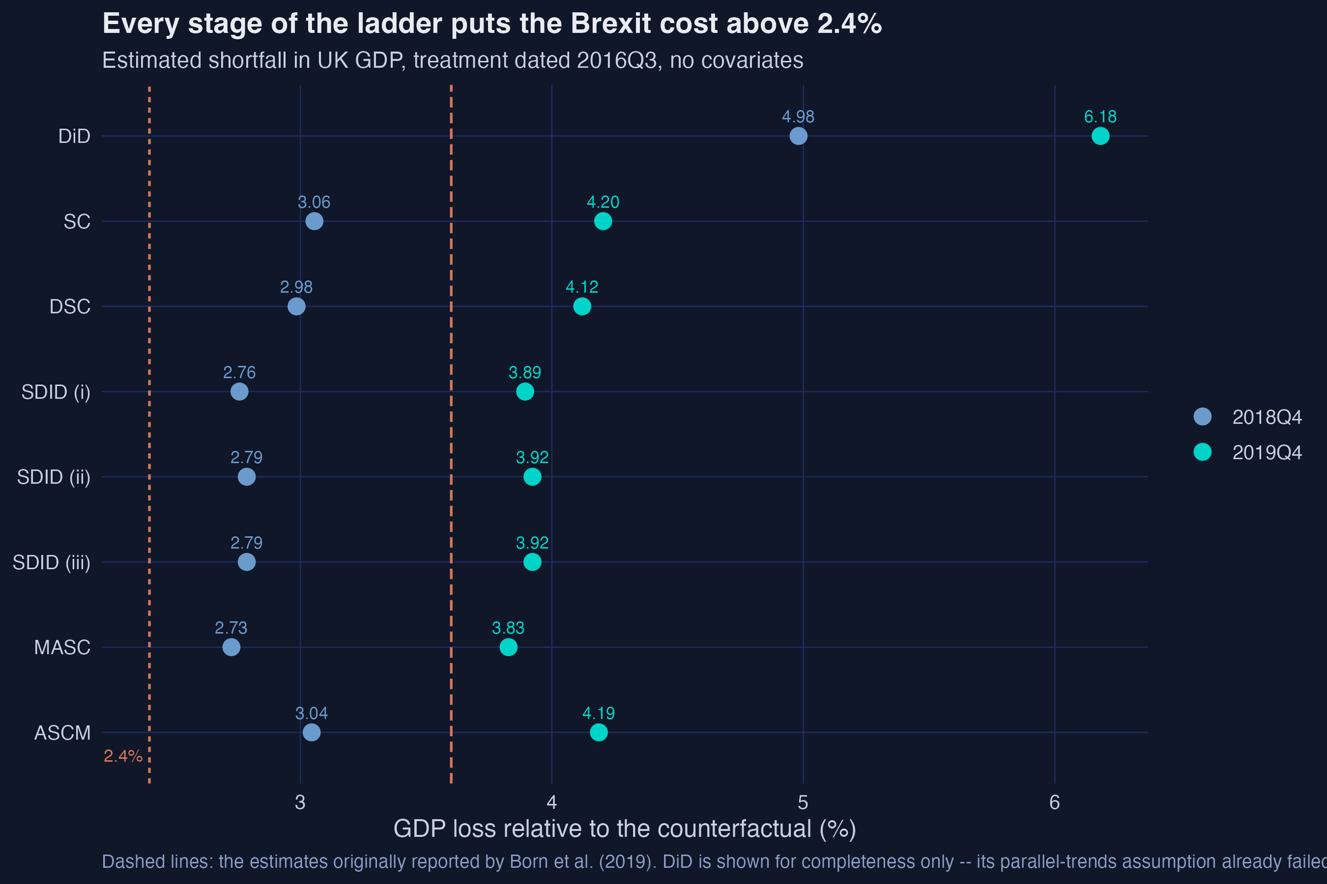
Every estimator’s 2018Q4 and 2019Q4 estimate, with Born et al.’s 2.4% as a dashed reference line.

2.73% to 3.06% at end-2018; 3.83% to 4.20% at end-2019.

Every stage of the ladder lands to the right of the published 2.4%.

Which stage? A fire drill

Re-date the treatment to each of twenty quarters when nothing happened. Every estimate is then pure error.

Method	RMSE	Median abs. error
SC	0.0089	0.0055
DSC	0.0087	0.0052
SDID (i)	0.0067	0.0016
MASC	0.0080	0.0045
ASCM	0.0086	0.0051
SDID (ii)	0.0134	0.0103
SDID (iii)	0.0134	0.0107

SDID (i) wins on every measure — and, as published, variants (ii) and (iii) look worst of all. Hold that thought.

Read as published, SDID (i) wins comfortably — a median absolute error of 0.0016 against plain SC’s 0.0055 — and variants (ii) and (iii) are twice as bad as plain SC. That is the basis for the source paper’s recommendation to use variant (i) in practice. Every number here reproduces the published table exactly.

But check the exam before trusting the ranking

The published table grades SDID (ii) and (iii) four quarters ahead and everyone else one quarter ahead.

Matched horizons, \(h = 1\):

SDID (i)	SDID (ii)	SDID (iii)
0.0067	0.0066	0.0066

The three variants are indistinguishable — the published ranking among them is an artefact of the horizon, not a property of the estimators.

What survives is the finding that matters more: at either horizon the whole SDID family beats every other stage, and the ordering below it is stable — SDID, then MASC, then ASCM, then DSC, then SC. Which variant supplies the time weights is simply not settled by this evidence; variant (i) remains the sensible default because it is the cheapest and needs no choice of post-treatment window.

Covariates make it worse

The dataset ships six covariates. Matching on them raises the placebo error:

• SC: 0.0089 → 0.0092
• DSC: 0.0087 → 0.0106

86 pre-treatment outcomes already encode the covariates (Kaul et al. 2022).

The six extra predictors add noise, not information.

With a pre-period this long, covariates cost precision and buy no identification.

Two things for the spoken version. First, the reconciliation with the literature: SC(B) — the Born specification, which scores covariates in both optimisation loops — reproduces the published 2.43% at 2018Q4 exactly. So the gap between the earlier published figure and everything on this ladder is the choice of estimator, not the data. Second, the exception: MASC’s placebo error clearly benefits from covariates, falling from 0.0080 to 0.0048; SDID and ASCM barely move. It is SC and DSC that are degraded.

And the optimiser matters more than you would think

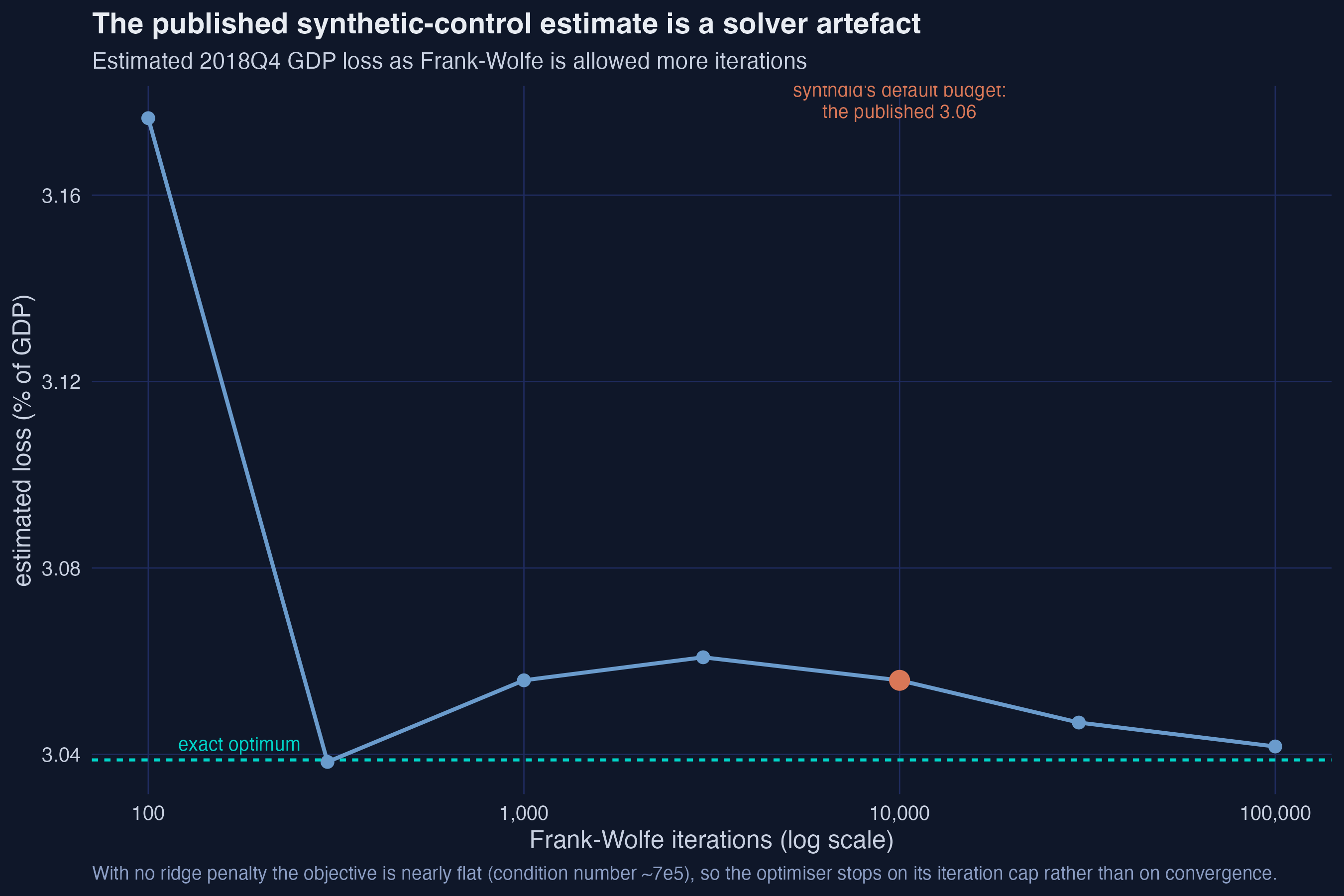
Estimated 2018Q4 loss against the number of Frank–Wolfe iterations, converging toward the exact optimum; the package default is marked in orange.

The published 3.06% is where Frank–Wolfe happens to be at 10,000 iterations. The true optimum is 3.04%.

A synthetic control estimate carries its solver’s fingerprint.

The strongest objection — and the answer

Objection. A 0.03 percentage-point spread cannot possibly rank estimators.

Response. True — which is why the placebo tournament, not the point estimate, does the ranking.

Pre-treatment fit cannot arbitrate between methods that all achieve it. Twenty fake treatment dates can.

The decomposition is durable; the leaderboard is not

1. The bias decomposition is the durable idea. The leaderboard is perishable.
2. Fit the ladder, not a stage. Report the cloud.
3. Run a placebo tournament — and check the horizons match.
4. Covariates are not free. With a long pre-period they may be redundant.

The rungs of this ladder are perishable; the question each rung answers is not.

Everything here replicates from one script and one CSV

Post · carlos-mendez.org/post/r_sc_dsc_sdid

Code · analysis.R (18 figures, full replication) · cheatsheet_R.R / cheatsheet_stata.do / cheatsheet_python.py (every estimator, one package call each)

Data · brexit_analysis.csv, loadable straight from GitHub

Replicates de Brabander, Juodis & Miyazato Szini (2025), Econometric Reviews 44(10), 1617–1646.

And the answer, with its error bars

Brexit cost the UK roughly 3% of GDP by end-2018, 4% by end-2019 — more than previously published.

The permutation p-value is 0.042 — the smallest 23 donors can produce.

A conventional 95% interval spans roughly 0.9% to 4.6%.

The point estimate is far better determined than the interval.

Those two lines answer different questions and should not be merged. The p-value is randomisation inference: how unusual is the United Kingdom among OECD countries. The interval comes from the synthdid placebo standard error of 0.0095 log points and speaks to sampling error. Only the first has a well-defined answer with one treated unit. Anyone quoting “Brexit cost 2.8%” without that interval is overstating what this design delivers.

Fit the ladder, not a stage — and publish the cloud, not the point.