Spatial Inequality and the Kuznets Curve

Is there an inverted-U? A synthetic replication in R

inverted-Udevelopment → spatial inequality

$2,100 / $31,000turning points

cubic n.s.within countries (panel FE)

Carlos Mendez

Nagoya University (GSID)

August 4, 2026

The Tension

Act I

Why do some countries have huge regional gaps and others almost none?

Kuznets and Williamson had an answer: rise, then fall.

Nobody could test it — the regional data barely exist.

Lessmann (2014) built them. We rebuild the whole exercise on synthetic data.

The hook: an old, intuitive hypothesis — Kuznets (1955) and Williamson (1965) — that was very hard to test, because testing it needs regional accounts for poor and rich countries, and those barely exist. Lessmann (2014) assembled them; the data are proprietary, so we rebuild the exercise on synthetic data calibrated to the paper. That keeps the whole pipeline open and reproducible, which is what makes it teachable.

Two pictures of the same question — and they disagree

Cross-section: a line declines, a quadratic bends, a cubic adds a high-income upturn.

The shape you see depends on the functional form you assume.

Plant the puzzle: the same scatter supports three different stories depending on the polynomial. We earn each curve in Act II, then resolve the between-vs-within tension.

Four estimators, one question — and they don’t all agree

• Measure it — the weighted coefficient of variation (WCV)
• Estimate it — cross-section OLS, panel fixed effects, two semiparametric checks
• The twist — the upturn is between countries, not within them

Same data, three shapes. Fixed effects settle which one is real.

The roadmap. The four estimators are cross-section polynomial OLS, two-way fixed effects with fixest, Robinson (1988) and Baltagi–Li (2002). Each asks the same question with fewer shape assumptions than the last. The payoff is the between-vs-within contrast at the end — that is where the deck is going.

The Investigation

Act II

We compute inequality, not assume it

\[\mathrm{WCV} = \frac{1}{\bar{y}}\left[\sum_{j} p_j\,(\bar{y}-y_j)^2\right]^{1/2}\]

Population-weighted spread of regional GDP per capita.

56 countries · 1980–2009 · 890 annual observations

A populous poor region counts; a tiny rich enclave barely moves it.

We simulate regions inside each country and compute the WCV from them, rather than taking an inequality index off the shelf. Here p_j is region j’s share of the country’s population and ybar is the country’s population-weighted mean regional income; the index is scale-free, so it compares a $400 economy with an $80,000 one. The synthetic panel has 890 annual country-year observations over 56 countries, 1980–2009 — close to the paper’s 915 / 56. The worked two-region example in the post gives WCV = 0.434.

Spatial inequality is related to personal inequality — but not the same

GINI = 0.31 + 0.21·WCV (t = 2.5, r = 0.32).

Regional gaps explain about a third of the cross-country variation in personal inequality — not all of it.

Motivates why we study the spatial dimension in its own right: the correlation is 0.32, close to the paper’s 0.324, so spatial inequality explains a real but partial share of personal inequality. A country can have high personal inequality with low regional inequality, or the reverse.

Cross-section: the inverted-U emerges with controls, and a cubic adds the upturn

Five specifications: bivariate → quadratic → +controls (inverted-U) → +cubic (N-shape).

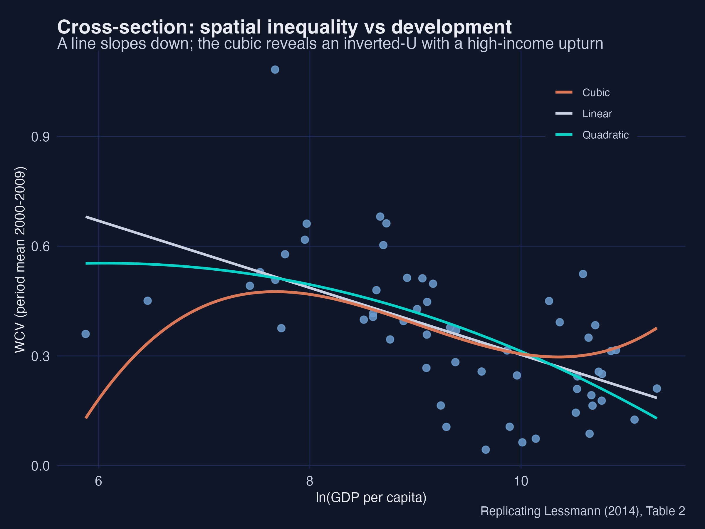
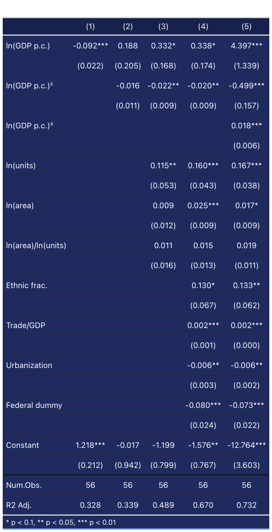
With controls the inverted-U appears (+0.34* / −0.02**); the cubic term adds the high-income upturn.

Column 1: the bivariate slope is negative (−0.092) — richer countries look more equal, but a straight line hides the structure. Column 4: +0.34 / −0.02 — the inverted-U. Column 5: cubic significant on all three income terms (+4.40*** / −0.499*** / +0.0184***) — the N-shape upturn. Every control carries the paper’s sign: trade and the number of regions raise spatial inequality; federalism and urbanisation lower it.

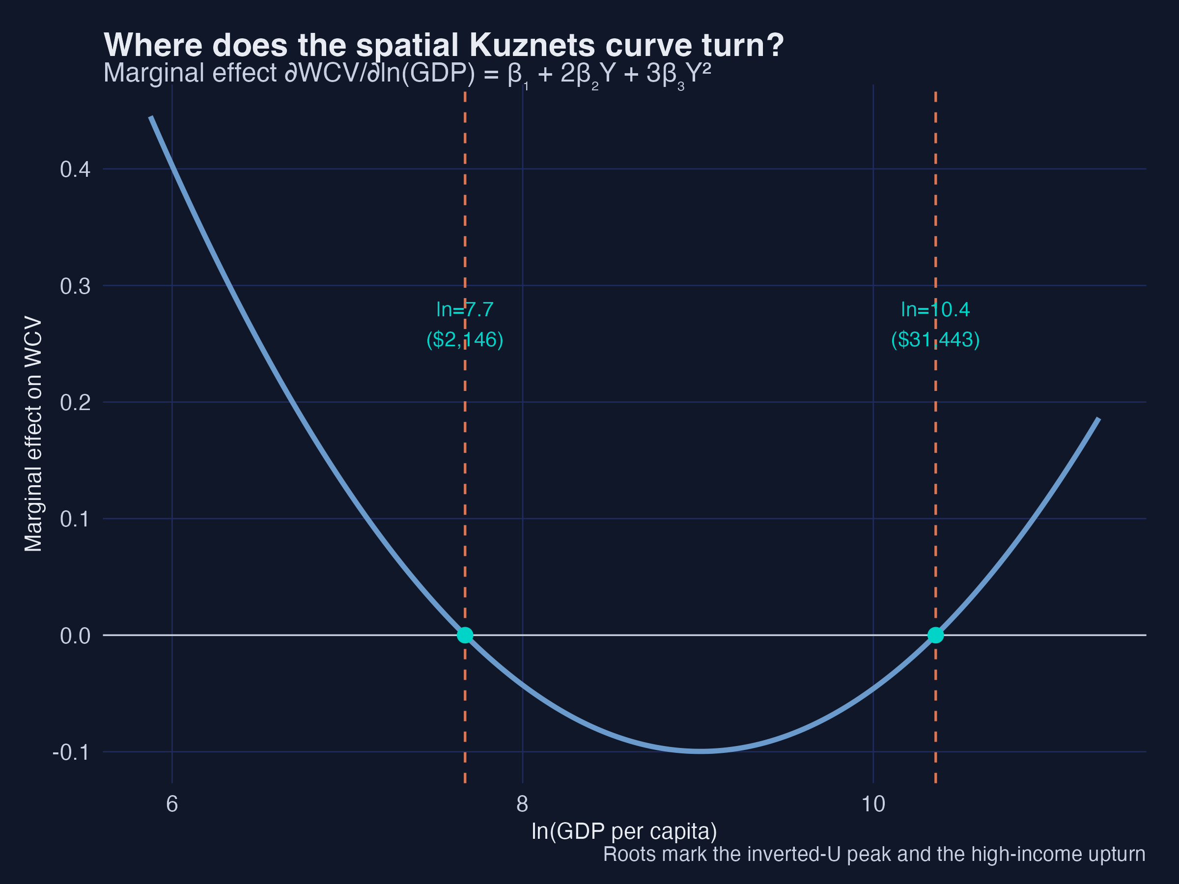
Where does the curve turn? Set the derivative to zero

Solving \(\partial \mathrm{WCV}/\partial \ln(\mathrm{GDP}) = \beta_1 + 2\beta_2 Y + 3\beta_3 Y^2 = 0\) gives a peak near $2,100 and a trough near $31,000.

Three phases: gaps widen up to $2,100, close until $31,000, then widen again.

Three phases: rise during the industrial take-off, fall through convergence, rise again at the post-industrial top. The roots come out in logs — ln(GDP) = 7.67 and 10.36 — so exponentiate to read them in dollars ($2,146 and $31,443). The paper reports ≈ $2,000 and ≈ $24,000.

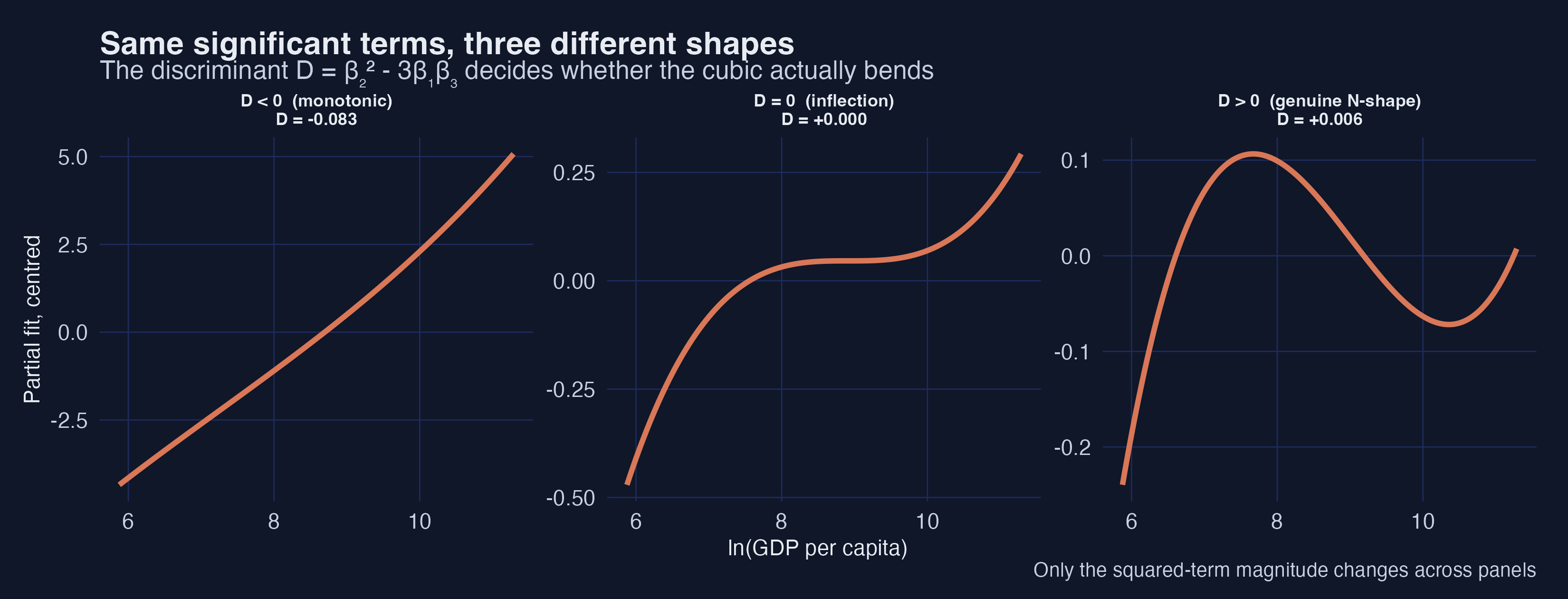
Significant ≠ a genuine bend — check the discriminant

The test: \(D=\beta_2^2-3\beta_1\beta_3\)

• \(D>0\) → two turning points · \(D=0\) → inflection only · \(D<0\) → monotonic
• Cross-section: \(D=+0.0055>0\), both turning points in range → genuine N-shape
• Panel cubic: insignificant, and a turning point falls far outside the data → no within-country bend

Significance says keep the term; the discriminant says whether the curve bends.

Say this aloud: all three cubic terms can be significant and the curve still not bend inside the observed range. Significance answers “does the data prefer keeping this term?”; the discriminant answers “does the fitted curve actually reverse?” — and a third check asks “does it reverse inside the data?” The cross-section passes all three (D = +0.0055, turning points $2,146 and $31,443 inside the observed $315–$82,653). The panel cubic fails on significance (t = −0.26) and, taken at face value, puts one turning point near $0.0003.

The discriminant decides the shape

Same significant terms, three shapes — only the discriminant tells them apart.

One number — the sign of \(D\) — separates a cubic that bends from one that merely curves.

Same sign pattern, vary only the squared term: D<0 monotonic, D=0 inflection, D>0 genuine N. In BMA the same trap reads “high PIP ≠ a genuine bend.” See the companion note (Mendez 2026).

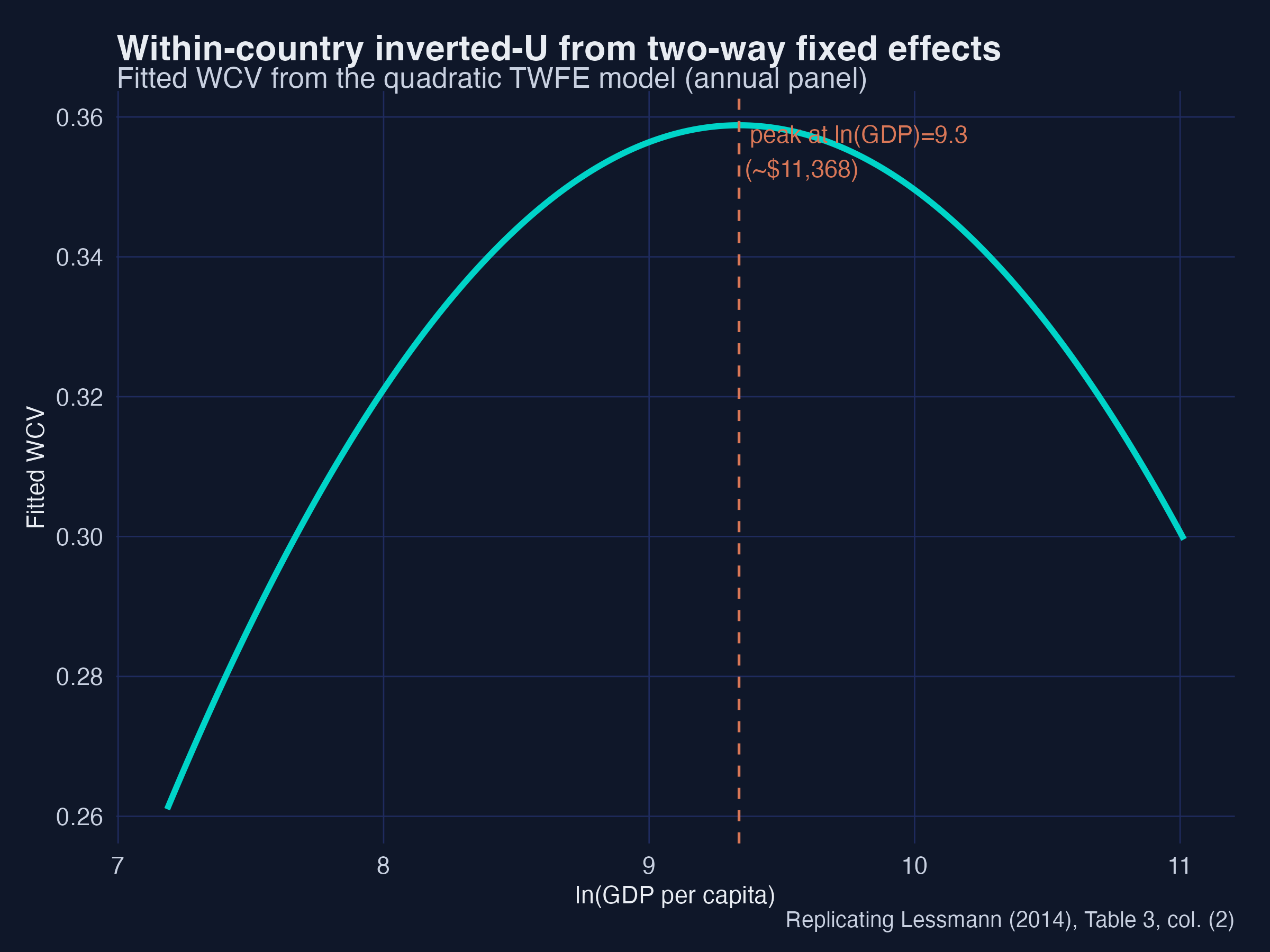
Fixed effects change the story, not just the standard errors

feols(wcv ~ lnGDP + I(lnGDP^2) + trade_gdp + urbanization |
            country + year, data = annual, vcov = "hetero")

• Within-country quadratic, two-way fixed effects (TWFE): +0.394** / −0.021** — a clean inverted-U
• Cubic term: insignificant — no within-country upturn

The upturn was a between-country artefact all along.

The vertical bar in fixest absorbs the country and year dummies; vcov = “hetero” reproduces the paper’s White standard errors (clustering by country is the modern alternative). Cross-section comparisons mix countries that sit at very different inequality levels for reasons unrelated to income; the panel compares each country with itself. The within-country cubic term is −0.0008 with t = −0.26 — no upturn. The 5-year averages give the same inverted-U, so this is not a business-cycle artefact.

Within a country, inequality peaks near $18,000 and then falls

Fitted WCV from the TWFE quadratic, peaking near $18,000.

Past the peak, a country’s regional gaps start to close as it keeps growing.

The fitted two-way fixed-effects quadratic peaks at ln(GDP) ≈ 9.8, about $18,000 per capita. Read it as the within-country trajectory: below the peak, growth widens regional gaps; above it, growth narrows them. This is the panel counterpart of the cross-section peak at $2,100 — a different question, so a different number.

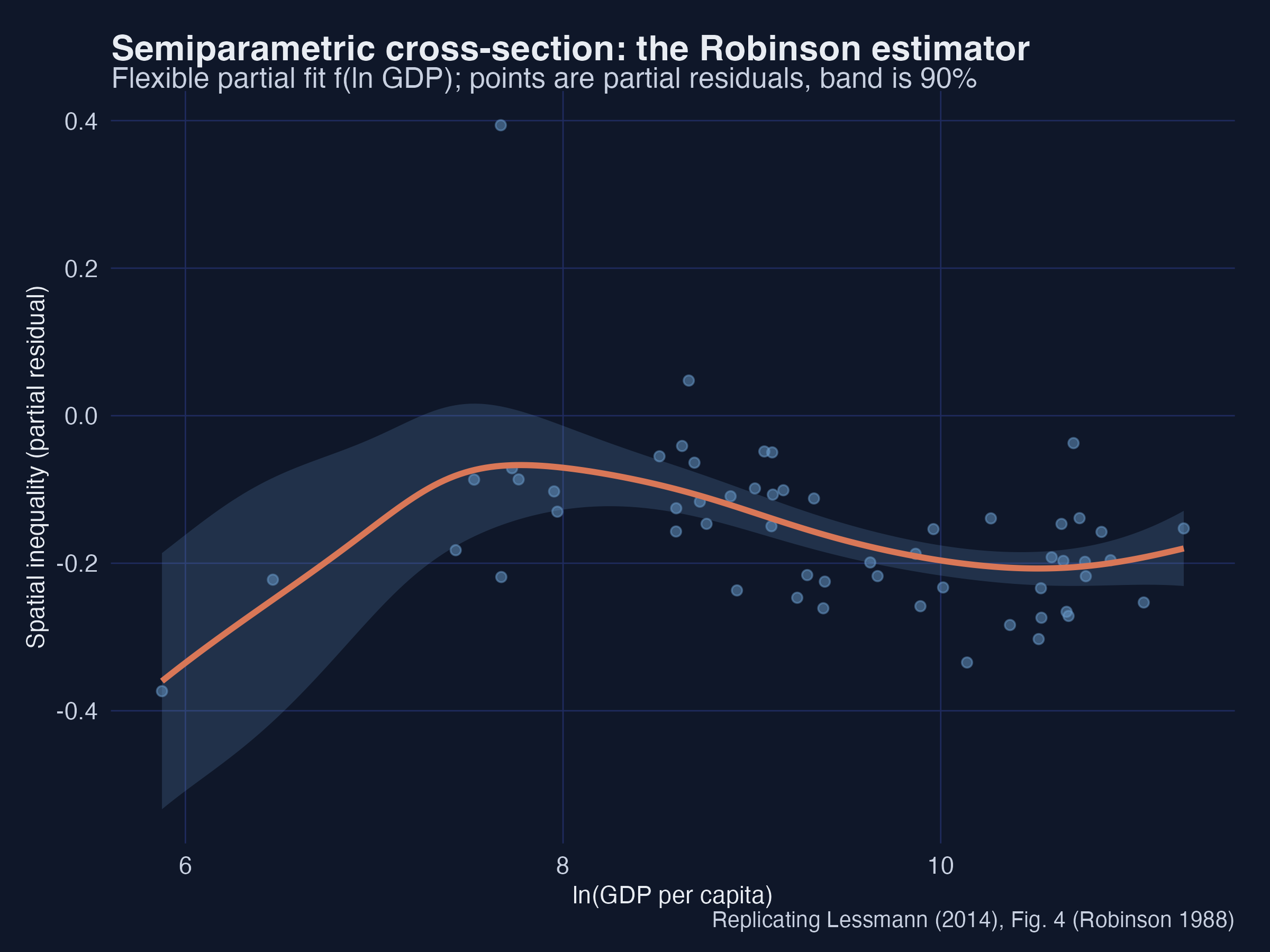
Semiparametric, no polynomial assumed — same shape

Robinson (1988) partial fit with a 90% band: inverted-U with a high-income upturn.

A curve that was never told to be a cubic traces the same shape.

Triangulation: a kernel-based estimator that never sees the word “cubic” recovers the same curve, and the 90% band widens where the data are sparse. The linear-part coefficients match the parametric ones, and np::npplreg returns the same point estimates as the hand-built double-residual version. Baltagi–Li (B-spline FE) agrees within countries — inverted-U, no upturn.

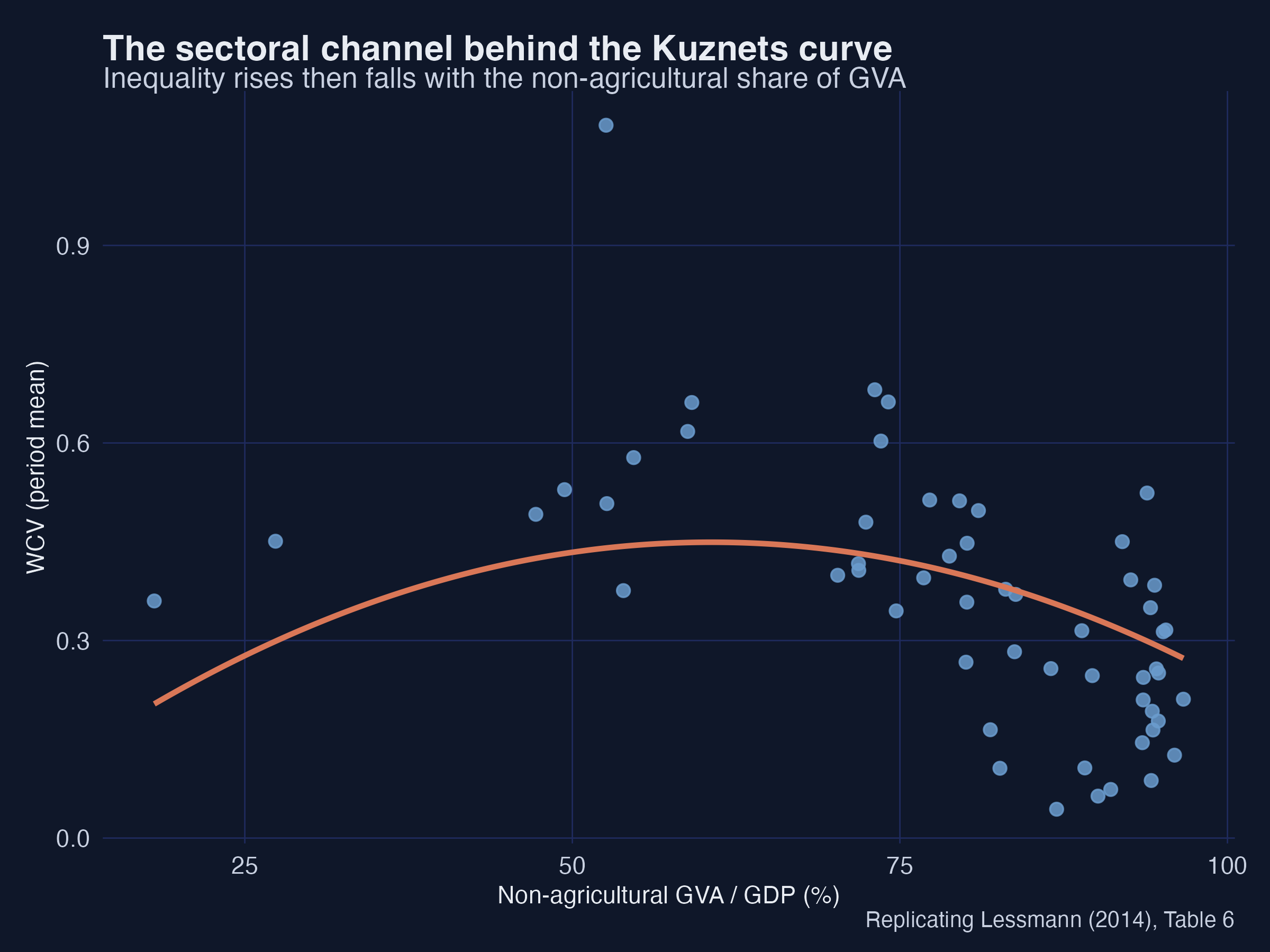
Structural change tracks the curve

Replace income with the non-agricultural share of output — the inverted-U returns.

Swap income for the non-agricultural share and the same inverted-U appears (+0.0165*** / −0.00014***).

Kuznets and Williamson argued that the real driver is structural change, with income only a proxy. As an economy industrialises a few regions capture the new activity and gaps widen; as the modern sector spreads, gaps close. Estimand note: this is an association, not identification — the whole study is descriptive, so “mechanism” here means a channel consistent with the data, not an estimated causal effect.

The strongest objection — and the answer

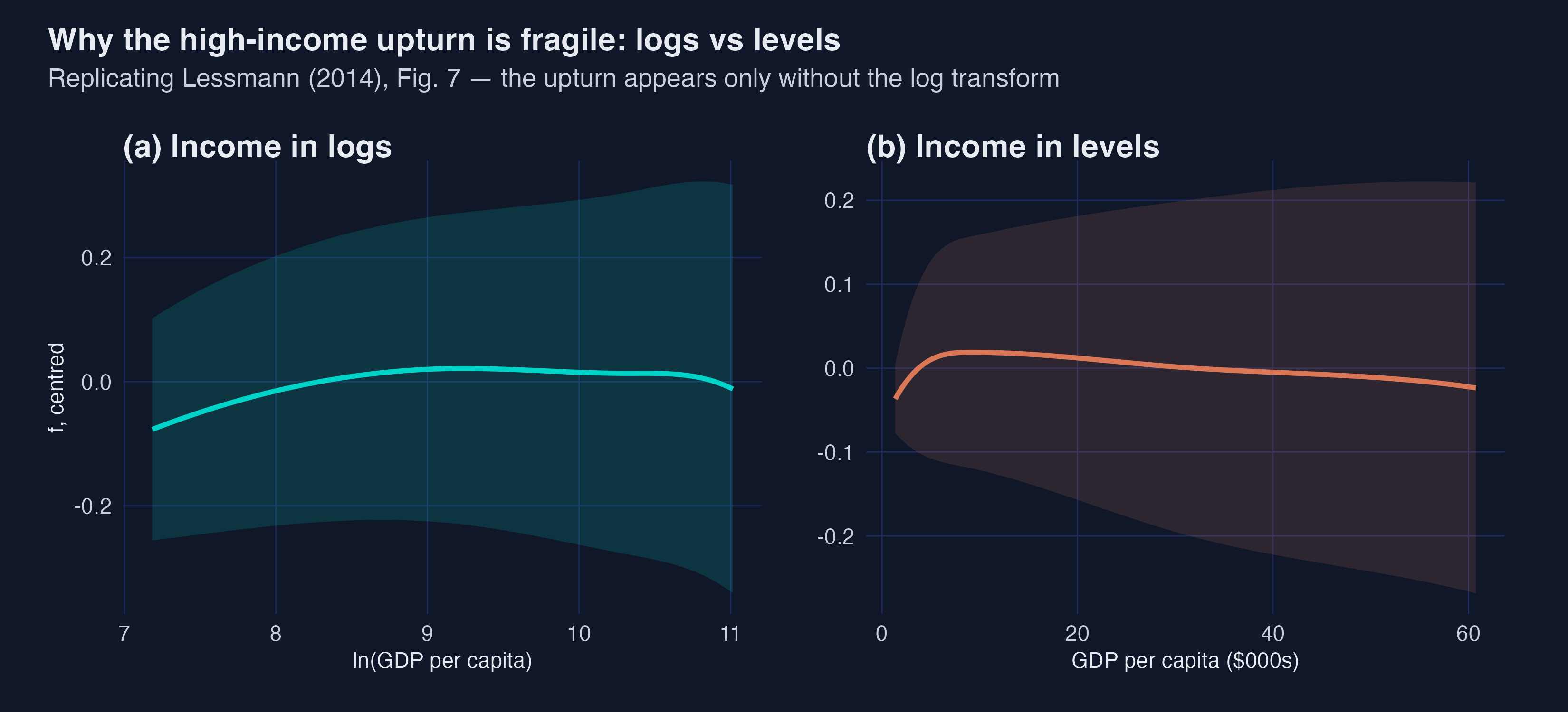
Objection. The high-income upturn is a measurement artefact — it shows up with income in levels and disappears in logs — and the data are synthetic anyway.

Response. Agreed on the upturn: we report it as fragile, not as a finding. The inverted-U itself survives logs, levels, fixed effects and both semiparametric estimators.

Steelman the critique from §11.4 of the post: the existence of the upturn is partly a measurement choice, which is exactly why Lessmann hedges it and why we hedge it too. It also weakens when the poorest countries are dropped. On the data: the synthetic world is calibrated to the paper’s published estimates, so it demonstrates the estimators — it is not independent evidence for the hypothesis.

The Resolution

Act III

Four estimators agree on the inverted-U — and disagree only on the upturn

• Inverted-U confirmed across cross-section OLS, panel TWFE, and two semiparametric estimators
• Turning points at ~$2,100 and ~$31,000 of GDP per capita
• The upturn is between-country, not within-country — fixed effects reveal it

All of it on synthetic data calibrated to Lessmann (2014) — a method demo, not new evidence.

The shape is robust; only the upturn depends on whether you look between or within countries.

The scorecard. Four estimators, one shape: the inverted-U appears in the cross-section with controls, within countries under two-way fixed effects, and in both semiparametric fits. They part company only on the high-income upturn, which the cross-section shows and the panel does not. Keep the caveat audible: these are engineered numbers that reproduce the paper’s estimates, so the exercise teaches the estimators rather than testing the hypothesis afresh.

The high-income upturn is real but fragile

It appears in income levels, vanishes in logs (and within countries).

Report the inverted-U with confidence; report the upturn with a caveat.

The post’s most important caveat (§11.4): with income in logs there is no high-income upturn; with income in levels a slight upturn reappears. So the existence of the upturn is partly a measurement choice. The robust finding is the inverted-U; the N-shape is real but fragile — which is why Lessmann hedges it and why we should too.

Wide regional gaps are a transitional stage of development — not a destination

The high-income upturn lives between countries, not within them.

Full tutorial, code, data and web app: carlos-mendez.org/post/r_kuznets

Reference: Lessmann, C. (2014). Spatial inequality and development — Is there an inverted-U relationship? Journal of Development Economics 106, 35–51. Synthetic data; pedagogical replication. The policy reading: gaps tend to widen during take-off and narrow as economies mature, but the transition can take decades, and the sectoral result points to the lever — human capital and connectivity in lagging regions.