Who Are My Neighbors?

Bayesian estimation of spatial weight matrices — and what changes when you stop assuming

8,010links estimated, not assumed

ρ = 0.713reproduced to 5 decimals

2.1×spillover vs own-region effect

Carlos Mendez

Nagoya University (GSID)

August 4, 2026

The seating chart you were handed

You have the transcript of the dinner.

You do not have the seating chart.

Spatial econometrics hands you the chart first — and asks you to trust it.

Open with the analogy, not the equation. The transcript is who laughed at which joke and who fell silent when. Spatial econometrics hands you the chart first — drawn from shared borders or straight-line distance — and asks you to trust it. The audience needs to feel the problem before seeing the machinery.

The Tension

Every spillover estimate is conditional on a matrix somebody chose

\[y_t = \rho W y_t + Z_{t-1}\beta + \varepsilon_t\]

• \(W\) says who is whose neighbour
• \(\rho\) says how strongly neighbours matter
• \(W\) is normally assumed, never estimated

If the map is wrong, every number downstream is wrong.

Emphasise: this is not a small auxiliary choice. It sits upstream of everything — the impacts, the spillover ratio, and the policy number at the end of the talk.

On this data, contiguity needs ten arbitrary decisions

Ten of ninety European NUTS-1 regions have no queen-contiguity neighbour at all:

Cyprus · Malta · Aegean islands · the Canaries · Åland · Corsica · Sicily & Sardinia · Azores · Madeira · Ireland

You patch each one by hand before the model will run.

None of those patches appears in the results table.

This is the single most persuasive slide for a sceptical audience. The “standard” approach already required ten undocumented judgement calls — attach each isolate to its nearest centroid by distance — before a single parameter was estimated. A contiguity matrix otherwise leaves all ten rows empty, which breaks row-standardization and effectively deletes those regions from the model.

The Investigation

Treat all 8,010 links as unknown parameters

	Assumed \(W\)	Estimated \(W\)
\(\rho\), \(\sigma^2\)	2	2
Slopes	4	4
Off-diagonal cells	0	8,010
Total unknowns	6	8,016
Observations	1,710	1,710
Obs per unknown	285	0.21

4.7 parameters per observation — the likelihood alone cannot do this.

Read the last row aloud. An assumed map leaves 285 observations for every unknown; estimating the map leaves about one observation for every five unknowns. That gap is why the prior — the next two slides — is doing the real work.

The prior is not a technicality — it is the method

\[p_{ij} \;\propto\; \omega_{ij} \;\times\; m(k_i)\]

Where links can be \(\times\) how many there are.

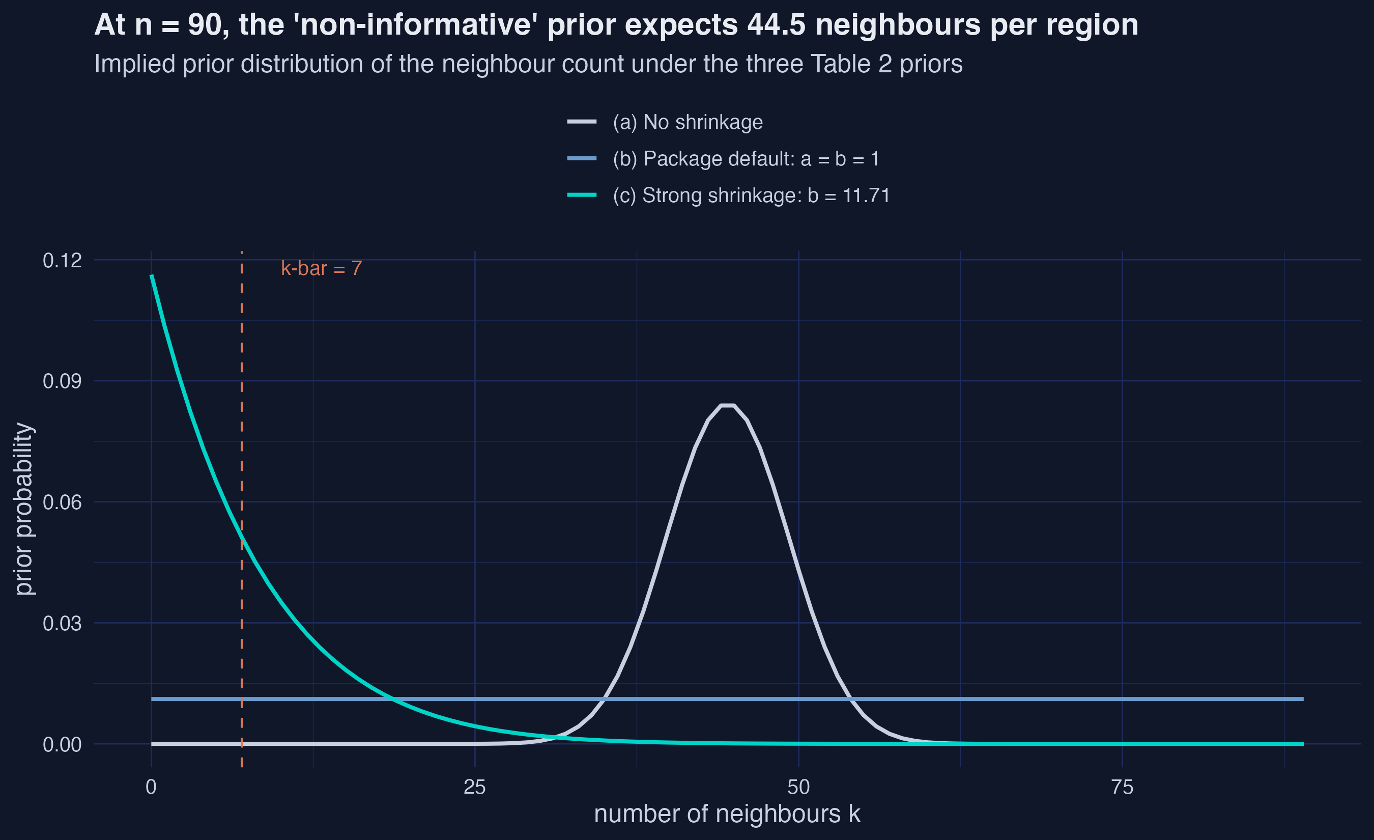
The trap: a “non-informative” flat prior expects 44.5 neighbours per region.

Every region wired to half of Europe.

The paper writes these hyperparameters with underbars; this deck drops them everywhere for legibility. The two factors are what matter — where a link may be, and how many links a region is expected to have. A flat weight is the natural thing to write if you want to impose nothing, but it implies a Binomial prior on the neighbour count centred at (n−1)/2. At n = 90 that is 44.5. The next slide shows what that choice actually asserts.

“Non-informative” means half of Europe

At n = 90 the flat and default priors expect 44.5 neighbours per region; only the shrinkage prior expects a sparse network.

The word “non-informative” describes the weight you type, not the belief you assert.

Grey bell centred at 44.5 is the flat prior. Teal spike at 7 is the anchored one. Same word, opposite belief. With only 19 time periods a prior centred on 44.5 would dominate the likelihood rather than be updated by it — which is exactly why the published application uses shrinkage.

One link at a time

A link is on or off, so conditional on everything else there are only two states to score:

\[p(\omega_{ij} \mid \Omega_{-ij}, \cdot, \mathcal{D}) \sim \text{Bernoulli}\left(\frac{\bar{p}^{(1)}_{ij}}{\bar{p}^{(0)}_{ij} + \bar{p}^{(1)}_{ij}}\right)\]

Score both, normalise, flip a weighted coin. Repeat 8,010 times per sweep.

The network is never solved whole — only one link at a time, given all the others.

Piano-tuning analogy: never solve the whole instrument, fix one string given the others. Each flip changes W, which changes the determinant. Sherman-Morrison rank-one updates make that cheap instead of O(n cubed) — which is why 8,010 links take minutes, not weeks.

The whole method is two function calls

kbar <- 7                                  # expected neighbours per region
b_pr <- ((n - 1) - kbar) / kbar            # 11.714  ->  link prob 7/89
AA   <- W_priors(n = n, W_prior = Wprior,
                 nr_neighbors_prior = bbinompdf(0:(n - 1),
                                                nsize = n - 1,
                                                a = 1, b = b_pr))

res_sarw <- sarw(Y = Y, tt = tt, Z = Z,
                 niter = 200, nretain = 100, W_prior = AA)

Every modelling decision lives in the prior object; sarw() only runs it.

The package is estimateW, on CRAN. W_priors() builds the beta-binomial sparsity prior anchored at seven expected neighbours; sarw() is the SAR panel sampler with W unknown. Two hundred iterations of which one hundred are retained is the paper’s own budget, reproduced deliberately — 350 seconds for the European panel. The full script ships with the post.

First, check it on a network we built ourselves

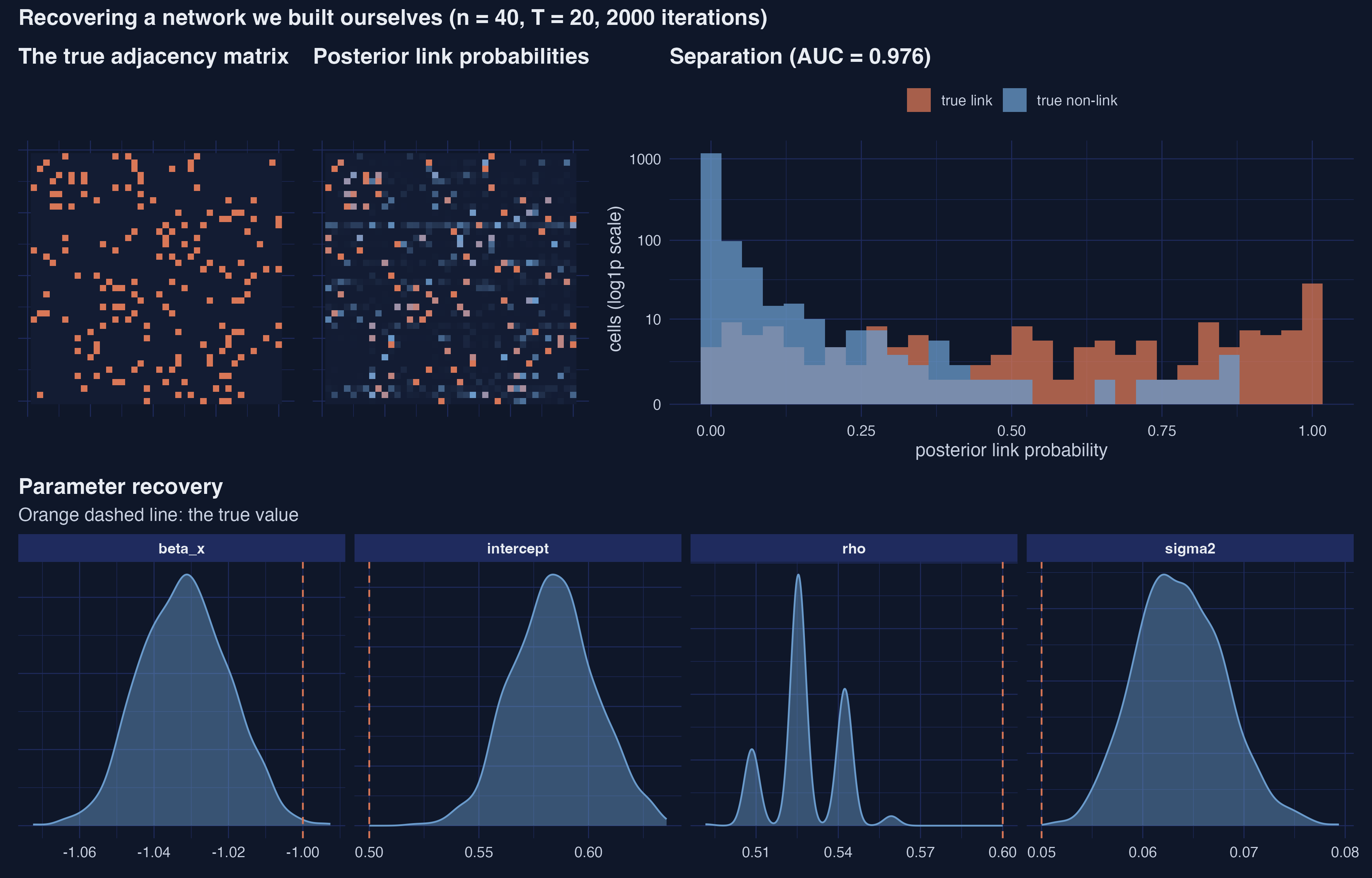
True adjacency, estimated link probabilities, the separation of true links from non-links, and each parameter’s posterior against its true value.

AUC 0.976 · 95.3% of 1,560 cells classified correctly

On a network whose answer we already knew, the sampler found it.

A driving test where you placed the cones — 40 units, 20 periods, four true neighbours each. Build trust before spending it on real data. The sampler is conservative: recall at the 0.5 cut is only 0.600 and the estimated mean degree is 3.05 against a true 4. That is the sparsity prior doing exactly what we asked of it.

But the intervals are not calibrated

	True	Estimate	95% interval	Covered?
\(\rho\)	0.600	0.528	[0.509, 0.542]	no
\(\sigma^2\)	0.050	0.064	[0.056, 0.073]	no
slope	−1.000	−1.032	[−1.053, −1.009]	no

The sparsity prior thins the network, and pulls \(\rho\) down with it.

Trust the structure. Hedge the intervals.

Two things compound. A sparser network has fewer channels for spatial transmission, so the model attributes less to rho — a real bias, not noise, and the price of the regularisation that made the problem estimable at all. On top of that an autocorrelated chain reports less uncertainty than it has earned, so the intervals are simply too narrow. One simulated dataset is not a Monte Carlo study; Krisztin and Piribauer run a proper one.

The published table reproduces exactly

Quantity	Paper	Ours	Verdict
\(\rho\)	0.71322	0.71322	exact
log initial GVA	−0.01692	−0.016922	exact
share high education	0.00044	0.000441	exact
av. indirect, initial GVA	−0.03972	−0.039723	exact

12 of 12 quantities exact to the five decimals printed.

Reproducing the published numbers is the licence to reinterpret them.

The exactness is conditional and worth naming: same seed, same package version, same RNG stream, same BLAS. Change any one of those and the fifth decimal moves. Everything after this slide is our own reading of the very same fitted object.

The model reconstructed national borders

Posterior link probability, ordered by group then country.

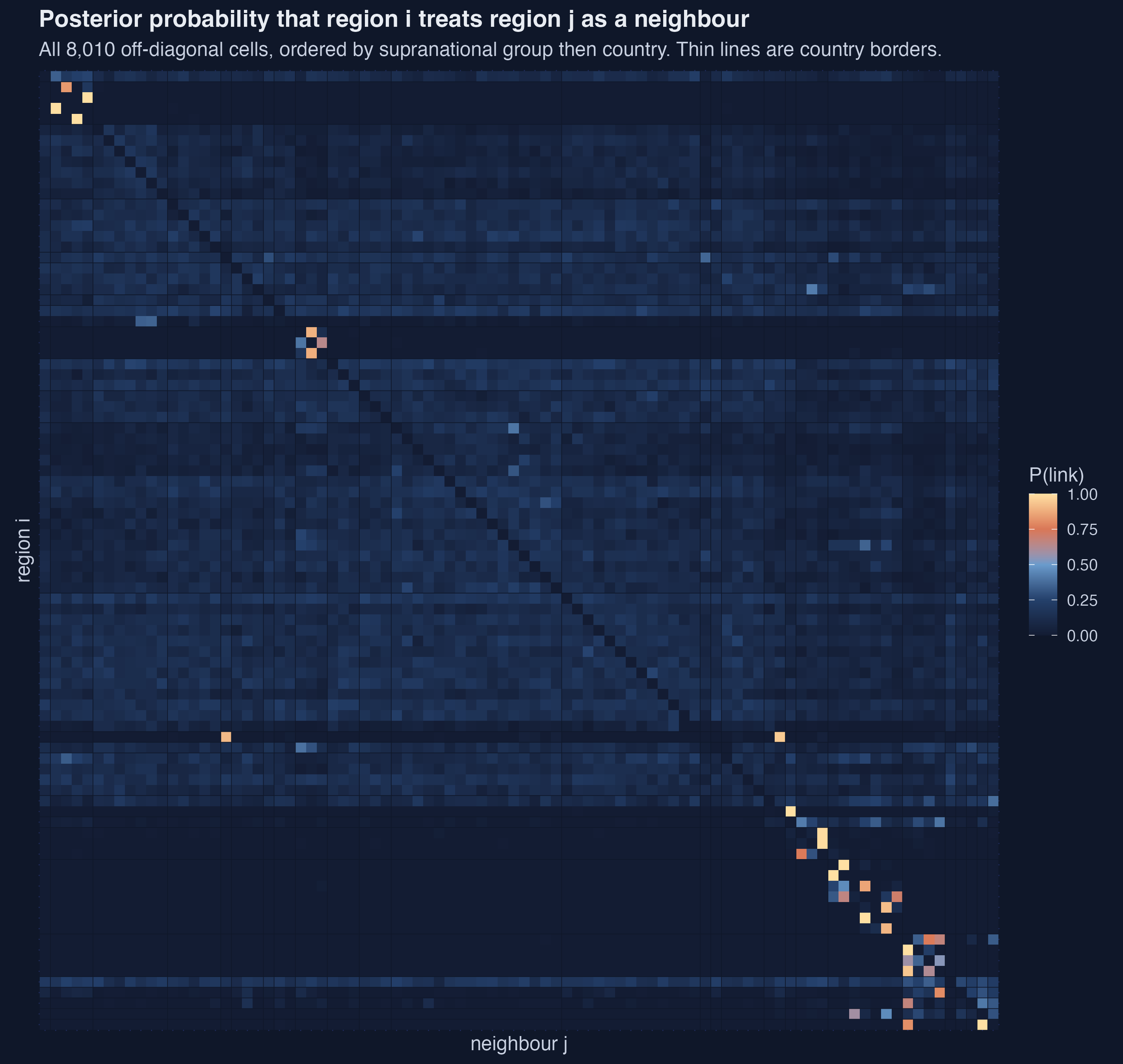
Regions place 35.6% of their neighbourhood weight on compatriots.

Chance would give 7.1%.

Nothing in the specification mentions countries — the model saw only growth, initial productivity and two education shares.

The bright blocks along the diagonal are the headline; the thin lines mark country borders. Five times more weight on compatriots than chance would predict, and twice as much on the supranational bloc. This turns the paper’s qualitative claim — that regions of the same country are more strongly interconnected — into a testable ratio.

Same country beats shared border

Comparator	AUC	Share of top links
Same country	0.753	30.2%
Queen contiguity	0.698	17.2%
7-nearest neighbours	0.631	23.9%

The strongest links average 921 km; a random pair averages 1,331 km.

Among the 33 links with probability \(\geq 0.5\): 60.6% share a border (14.2× enrichment) against 75.8% same-country (10.6×).

Nationality organises the whole ranking; geography owns the links the data are certain about.

Two questions, two answers, and the post reports both rather than only the one that supports the headline. Across the full ranking of 8,010 pairs, “same country” discriminates better than “shares a border” — AUC 0.753 against 0.698. Restrict to the 33 pairs the model is most confident about and the picture tilts back toward geography: 60.6 per cent of them share a border, an enrichment of 14.2 times over a 4.3 per cent base rate, while 75.8 per cent are within a country, an enrichment of 10.6 times. “What organises this network?” and “what does the model know for sure?” are different questions.

Long arcs, not short ones, carry the network

The strongest 10% of estimated links as arcs between region centroids: teal where the pair also shares a border, orange where it does not.

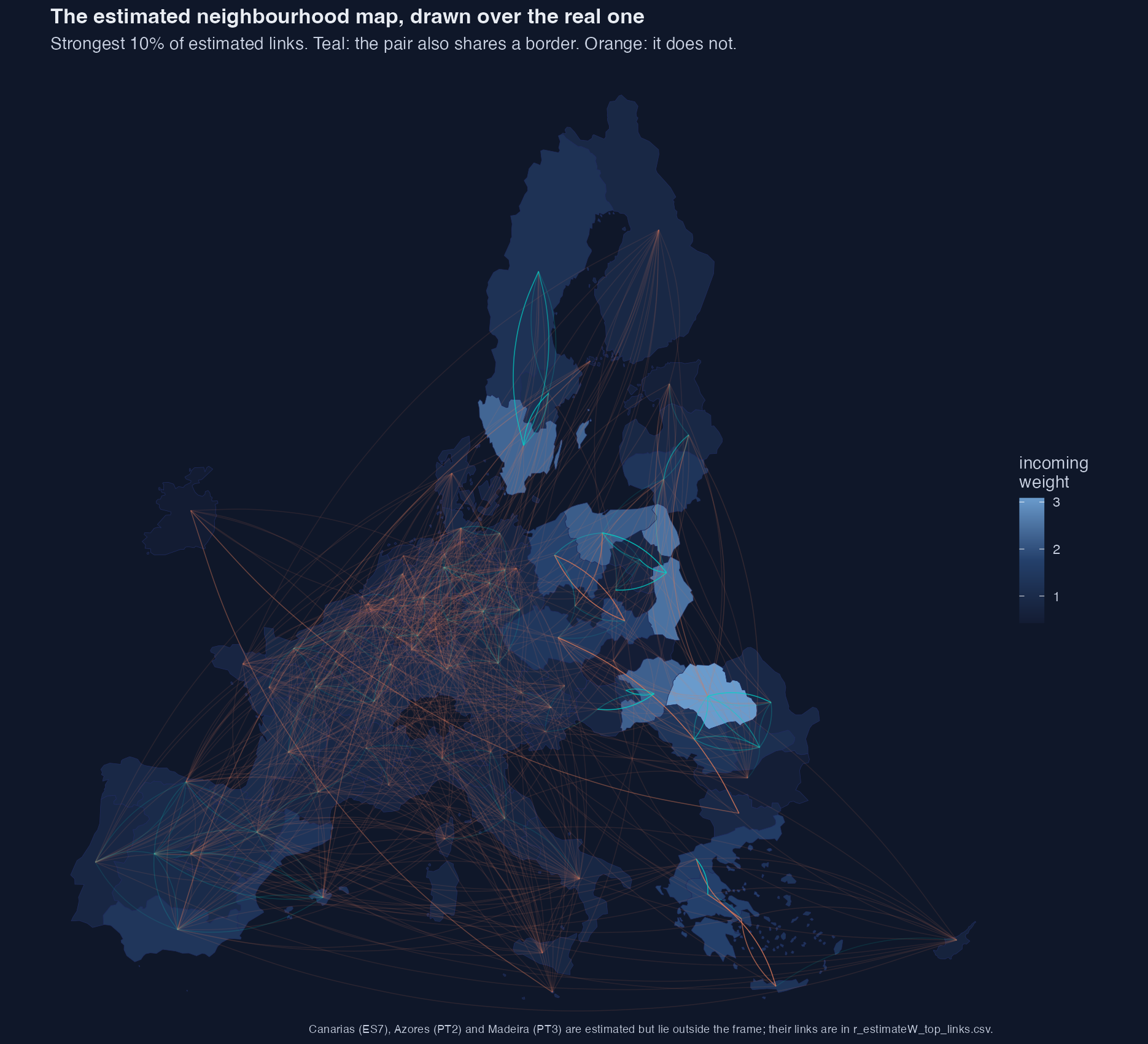
Teal — the pair also shares a border.

Orange — it does not.

Long orange arcs dominate: Bulgaria to Czechia, Iberia to the Baltic, Greece to Ireland.

Were the estimated network essentially contiguity, this would be a mesh of short teal arcs hugging borders.

This figure makes the point better than any table — give the room a beat to look before you speak. Whether those long links represent trade, migration, shared exposure to European business cycles or common institutional shocks is a question this model cannot answer; the “what this cannot tell you” slide returns to it.

Three maps, three answers

	Estimated	Queen	7-NN
\(\rho\)	0.713	0.607	0.719
High education, total	0.00153	0.00066	0.00074
Indirect ÷ direct	2.11	1.20	2.20

Every sign survives. Every magnitude moves.

The data-chosen map more than doubles the total education effect.

The same SAR specification, the same data, three neighbourhood maps — nothing changes but W. A referee asking “would your story change under a different W?” gets a reassuring answer on signs and an uncomfortable one on magnitudes. Note the mechanical pattern in rho: the sparsest map, queen contiguity at 3.8 neighbours, gives the lowest value; kNN-7 at exactly seven gives the highest; the estimated map at 6.47 lands between them.

The Resolution

Why that matters for policy

2.11 under the estimated map. 1.20 under contiguity.

Most of the education return leaks across borders — or only about half does. Same data, different map.

A region that raises tertiary attainment is associated with about twice as much growth outside its borders as inside them. Whoever funds the universities captures roughly a third of the measured return. Under contiguity that ratio is 1.20, not 2.11 — a materially different co-funding decision for a ministry choosing how much of a regional skills programme to pay for from a national or European budget.

What this cannot tell you

Bulgaria → Czechia at probability 1.0 says one thing only: residual co-movement fits better with that link than without it.

It does not mean trade, commuting, or FDI.

With \(T = 19\), genuine transmission and shared exposure to common shocks are indistinguishable.

Do not let anyone leave the room thinking this is a causal network. That probability is also conditional on a prior that expected seven neighbours. Two regions responding identically to a common European shock look connected to this model even if nothing flows between them. Naming the mechanism requires data on the mechanism.

26.5 effective draws bound what we can claim

• ESS(\(\rho\)) = 26.5 of 100 retained draws (Geweke \(z = -3.74\)), so a link probability is quantized to 0.01
• Posterior means are stable across chains and budgets; SDs, intervals and link rankings are not
• Practical ceiling: about 300 regions
• \(k = 7\) is a researcher choice — report a sweep, not a number

Report the point estimates. Hedge everything that has a width.

An effective sample size of 26 supports a mean; it does not support a credible interval you would defend in a referee report. With 100 retained draws a link seen three times is indistinguishable from one seen once, so the boundary of the “strongest 10 per cent” sits in the noisy region. The paper writes the prior anchor with an underbar; this deck drops it. Prior sensitivity here is the first thing a referee should ask about.

The map is a parameter

Every spatial result you have read is conditional on a map somebody chose — and it does not have to be.

Full tutorial, code and replication bundle: https://carlos-mendez.org/post/r_estimatew/

Land on the thesis and stop. The invitation, if there is time for one, is the tutorial and the replication bundle — everything in this talk runs end to end from it.