Introduction to the Synthetic Control Method in Python with mlsynth

Did Proposition 99 reduce cigarette sales in California?

−18.98ATT, packs per capita per year

1 of 39placebo rank, p = 0.026

5 of 38donor states in the recipe

Carlos Mendez

Nagoya University (GSID)

October 5, 2026

The Tension

Act I

Act I sets up the puzzle that the method must solve. Cigarette sales were already falling across the country when California launched its program in 1989. We first show why the obvious comparisons fail, and then we lay out the plan of the talk.

Cigarette sales fell everywhere, so did Proposition 99 change anything?

In November 1988, California voters approved Proposition 99: a tax increase of 25 cents per pack from January 1989, plus anti-smoking education.

Average sales in California fell from 116.21 packs per capita in 1970–1988 to 60.35 in 1989–2000. Yet the average donor state also fell, by 28.51 packs, without any program.

A before-and-after comparison mixes the program with a national decline.

Proposition 99 raised the state cigarette tax by 25 cents per pack and funded anti-smoking education. Sales in California then fell steeply, from an average of 116.21 packs per capita over 1970–1988 to 60.35 over 1989–2000. Over the same two periods, however, the average of the 38 donor states fell by 28.51 packs. Part of the drop in California would therefore have happened anyway. Our question is counterfactual: how much lower were sales in California because of the program?

Before you look: did California move with the average state before 1989?

In 1970, California sold 2.92 packs per capita more than the average of the 38 donor states. How large is the gap in 1988, the last year before the program?

A.  Smaller: the two series converge

B.  Similar: the average tracks California closely

C.  Far larger: California falls well below the average

Ask the room to commit before the figure appears. Give the room 20 seconds, and then take the vote. Answer on the next slide: C. California sat 23.72 packs below the donor average in 1988, after starting 2.92 packs above it in 1970. A comparison with the average would therefore credit Proposition 99 with a relative decline that began long before 1989. (AhaSlides interactive follows.)

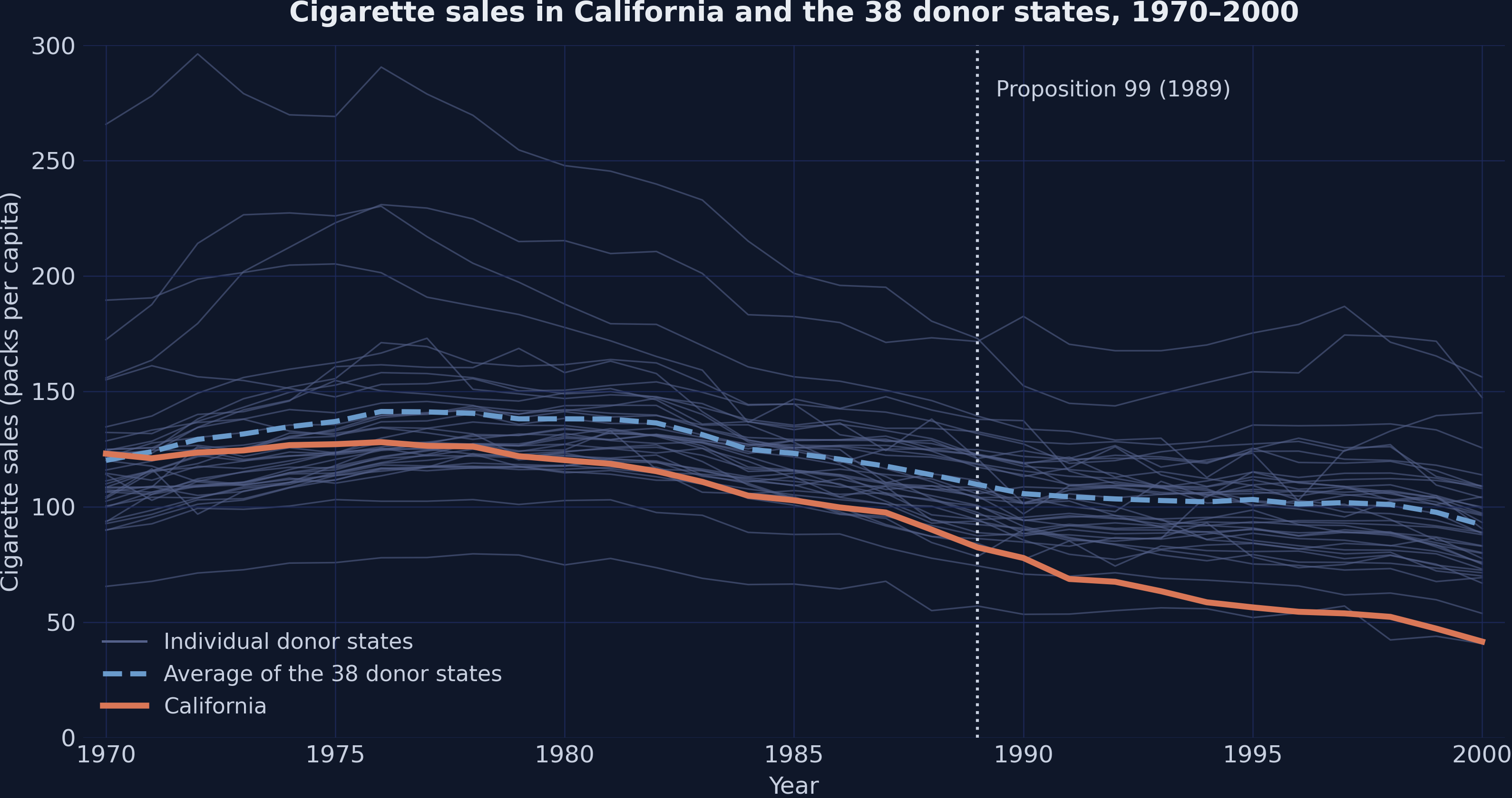
The average state is a poor twin: California was already falling faster

California (orange), the 38 donor states (gray), and their average (dashed blue), 1970–2000.

By 1988, California sat 23.72 packs below the donor average, so the simple average fails before the program starts.

The answer to the vote: C. The two series were close in 1970, at 123.0 against 120.08 packs. By 1988, California sold 90.1 packs against 113.82 for the average, a gap of −23.72 packs. The simple average gives every donor the same voice, and 25 of the 38 donors sold more than California over 1970–1988. The naive difference-in-differences estimate of −27.35 packs therefore rests on parallel paths that these years contradict.

The plan: build a synthetic California in mlsynth, then try to break it

• Data: 39 states from 1970 to 2000, and one treated state
• Method: a weighted recipe of donor states and the gap it leaves
• Tool: one mlsynth dictionary and one call to fit()
• Tests: placebos in space and in time, and leave-one-out refits
• Checks: the Stata benchmark, three other estimators, and five misreadings

Five times along the way, the room predicts the result before the reveal.

This is a teaching deck, so we signpost the route. Act II builds synthetic California and reads its weights, its fit, and its gap. Act III tries to break the result with placebo tests, leave-one-out refits, and other estimators. Five cue slides on a blue background ask the room to predict before each reveal, and on AhaSlides each cue is followed by a live quiz.

The Investigation

Act II

Act II builds the synthetic control one step at a time. We start with the data and the estimand, state the weight problem, and write the configuration that mlsynth needs. The act ends with the main estimate and a gap that widens through the 1990s.

The lab: 39 states, 31 years, one treated state, and one estimand

• Panel: 39 US states from 1970 to 2000, or 1,209 state-year rows
• Outcome: cigarette sales per capita, in packs
• Treated: California from 1989; donors: the other 38 states
• Predictors: four covariates averaged over 1980–1988, plus sales in 1975, 1980, and 1988

The estimand is the ATT: the effect of Proposition 99 on California alone, over 1989–2000.

The data are the panel of Abadie, Diamond, and Hainmueller (2010), the same file as the Stata edition. The panel is balanced, with 31 rows for each state. The original authors had already removed states with large tobacco programs or large tax increases, such as Arizona, Massachusetts, and Oregon. The four covariates are log GDP per capita, the share aged 15–24, the retail price of cigarettes, and beer consumption. Beer data start only in 1984, so the beer average over 1980–1988 rests on 1984–1988 alone. The method estimates what Proposition 99 did in California, not what it would do in Nevada or Texas.

A synthetic control is a weighted recipe of donor states

\[\min_{w_2, \ldots, w_{J+1}} \; \sum_{m=1}^{k} v_m \Big( X_{1m} - \sum_{j=2}^{J+1} w_j X_{jm} \Big)^2\]

\[\text{subject to} \quad w_j \geq 0 \quad \text{and} \quad \sum_{j=2}^{J+1} w_j = 1\]

Unit 1 is California, units 2 to 39 are the \(J = 38\) donors, and \(v_m\) sets the cost of a mismatch on predictor \(m\) of \(k = 7\).

Weights that are nonnegative and sum to one interpolate between donors; they never extrapolate beyond them.

Equation 1 chooses nonnegative donor weights that sum to one. These weights make synthetic California resemble California on each of the seven predictors before 1989. Because the weights form a convex combination, synthetic California can sell neither more than the highest donor nor less than the lowest donor. In 1988, California sold 90.1 packs, inside the donor range from 55.0 packs in Utah to 180.4 packs in New Hampshire. A convex combination can therefore reach it.

The predictor weights are not fixed in advance. An outer search chooses them so that the synthetic path also reproduces sales in California from 1970 to 1988. Many different predictor weights can lead to the same donor weights, a point that returns on a later slide.

The effect is the gap between California and its synthetic twin

\[\hat{Y}_{1t}^{N} = \sum_{j=2}^{J+1} w_j^{\ast} Y_{jt} \qquad\qquad \hat{\tau}_t = Y_{1t} - \hat{Y}_{1t}^{N}\]

\[\widehat{\mathrm{ATT}} = \frac{1}{T_1} \sum_{t=1989}^{2000} \hat{\tau}_t \qquad \text{with } T_1 = 12\]

The superscript \(N\) marks sales without the program, and a negative ATT means fewer packs than in synthetic California.

Once the weights are known, the counterfactual is simple arithmetic: a weighted average of donor sales.

Equation 2 applies the optimal weights to the sales of the donors in each year. The gap then subtracts this synthetic path from actual sales in California. Equation 3 averages the 12 yearly gaps from 1989 to 2000 into one number, the ATT. In mlsynth, these objects are res.counterfactual, res.gap, and res.att. Exercise 2 of the post rebuilds the synthetic path by hand and matches res.counterfactual up to floating-point error.

One configuration dictionary drives every mlsynth estimator

config = {
    "df": panel, "outcome": "cigsale", "treat": "treated",
    "unitid": "state", "time": "year",
    "covariates": COVARIATES,       # four covariates, three lags
    "covariate_windows": WINDOWS,   # 1980–1988, or one year per lag
    "backend": "mscmt",             # nested search over V and W
    "canonical_v": "min.loss.w", "seed": 42,
    "inference": False, "display_graphs": False,
}
res = VanillaSC(config).fit()       # res.att, res.donor_weights, res.gap

One dictionary describes the data and the settings, and one call to fit() returns the result object.

The mlsynth library organizes every estimator around one pattern: a dictionary of settings, an estimator class, and a call to fit(). Five keys describe the data, two keys describe the predictors, and the remaining keys choose the algorithm. The backend mscmt runs the nested search over the predictor weights V and the donor weights W, and the seed fixes its global search. The fit takes about one second, and the key inference stays off until the placebo test, because it would add 38 placebo fits.

The library validates the dictionary with pydantic before it computes anything. A misspelled key such as covariate_window therefore raises an MlsynthConfigError instead of failing silently. One trap remains in version 1.0.0: if every predictor spans the same years, the library first drops every year in which any predictor is missing. The lagged sales therefore receive their own one-year windows.

Before you look: how large is the share of Utah in the recipe?

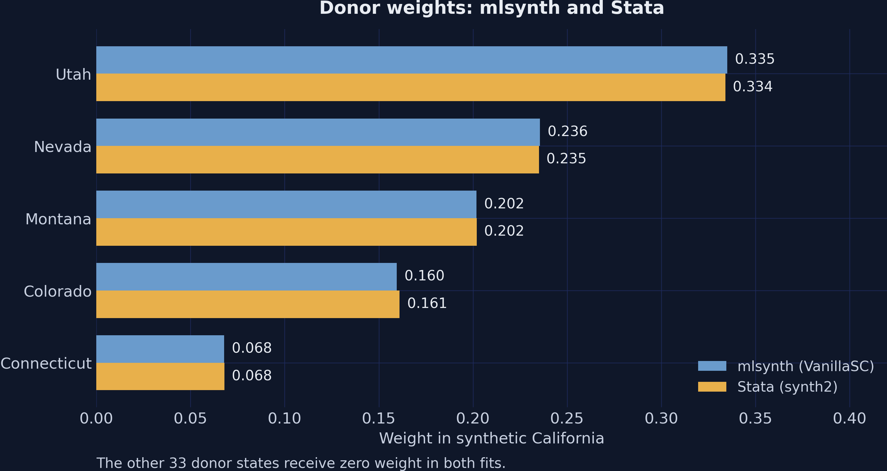
Five of the 38 donor states receive positive weight, led by Utah, the state with by far the lowest sales. How much of synthetic California does Utah supply?

A.  More than half: Utah alone is nearly the whole recipe

B.  About one third: the other four shares differ widely

C.  About one fifth: the five shares are nearly equal

Ask the room to commit before the weights appear. Give the room 20 seconds, and then take the vote. Answer on the next slide: B. Utah receives 0.335, about one third of the recipe. The other four shares range from 0.236 for Nevada to 0.068 for Connecticut, and the other 33 states receive exactly zero. (AhaSlides interactive follows.)

Five states build synthetic California, led by Utah

Donor weights of mlsynth (blue) and Stata (gold); the other 33 donor states receive zero weight in both fits.

Utah supplies one third of the recipe, and 33 of the 38 donors receive exactly zero.

The answer to the vote: B. The recipe is Utah (0.335), Nevada (0.236), Montana (0.202), Colorado (0.160), and Connecticut (0.068). Utah earns the largest share, because its low sales pull the weighted average down toward the level of California. The weights of mlsynth and Stata differ by less than 0.002 for every donor, so the two programs found the same recipe. Nevada is the only donor that borders California, so cross-border purchases could inflate its sales.

Before you look: will mlsynth and Stata agree on the predictor weights?

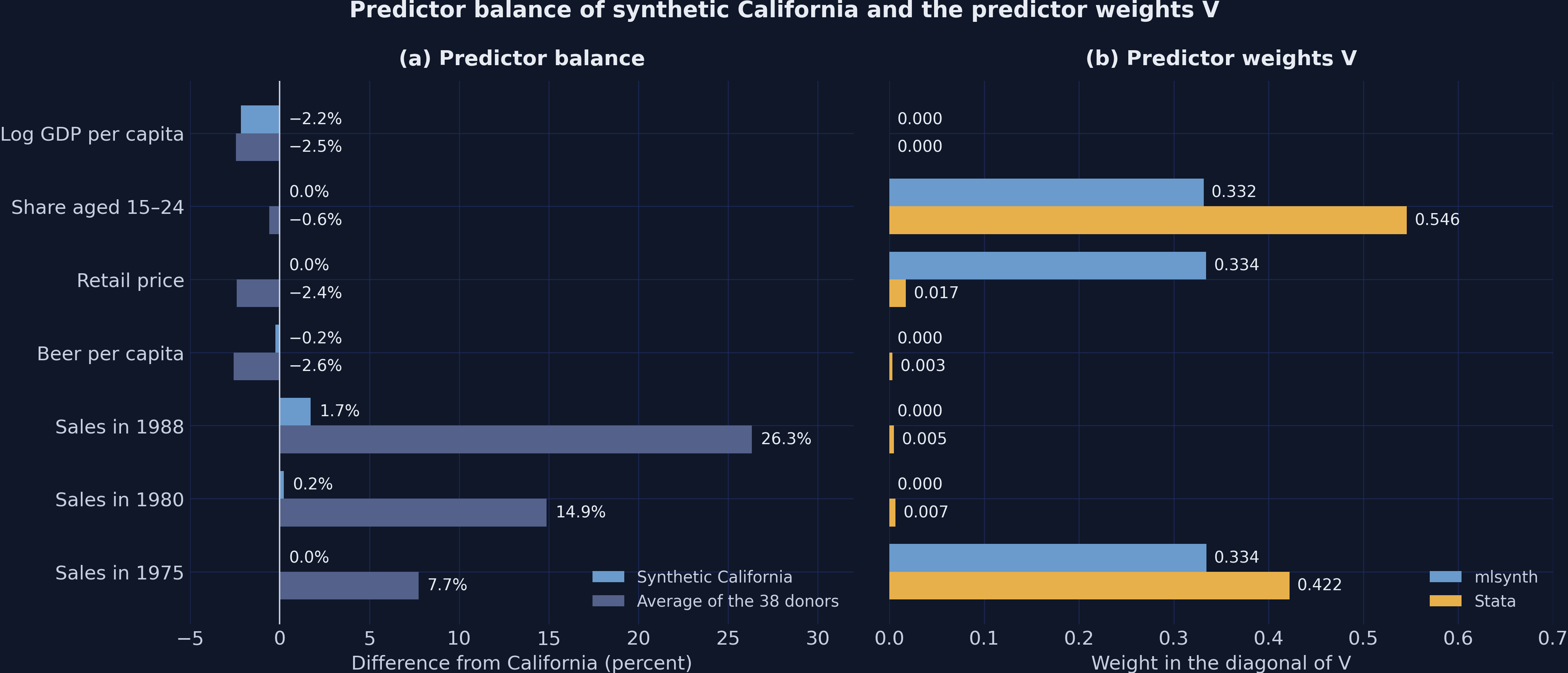
The two programs agree on the donor weights within 0.002. Stata puts 0.546 of the predictor weights on the age share and 0.422 on sales in 1975. What will mlsynth report?

A.  Very different predictor weights, yet the same donor weights

B.  The same predictor weights, since equal donor weights require them

C.  Different predictor weights, so one program must contain an error

Ask the room whether equal donor weights imply equal predictor weights. Give the room 20 seconds, and then take the vote. Answer on the next slide: A. The mlsynth fit puts about one third of V on each of the age share, the retail price, and sales in 1975. Both V vectors lead to almost the same donor weights, so V is not identified. (AhaSlides interactive follows.)

The same donor weights \(W\) arise from very different predictor weights \(V\)

(a) Percent gaps from California on the seven predictors; (b) the predictor weights \(V\) of mlsynth (blue) and Stata (gold).

Report \(V\) for transparency, but never rank predictors by it.

The answer to the vote: A. In mlsynth, the age share (0.332), the retail price (0.334), and sales in 1975 (0.334) each receive about one third of the predictor weights. These are exactly the three predictors that synthetic California matches with a gap of zero. Stata instead puts 0.546 on the age share and 0.422 on sales in 1975, yet both programs reach almost the same donor weights. When a few predictors are matched exactly, many V select the same W, so the data cannot single out one set of predictor weights. Exercise 6 of the post feeds the Stata V into the inner problem and recovers the Stata donor weights.

Panel (a) shows what the weights buy. On sales in 1988, the donor average misses California by 26.33 percent, while synthetic California misses by only 1.72 percent. Income is the exception, because its gap of −2.16 percent compares logarithms and implies a GDP per capita about 20 percent lower.

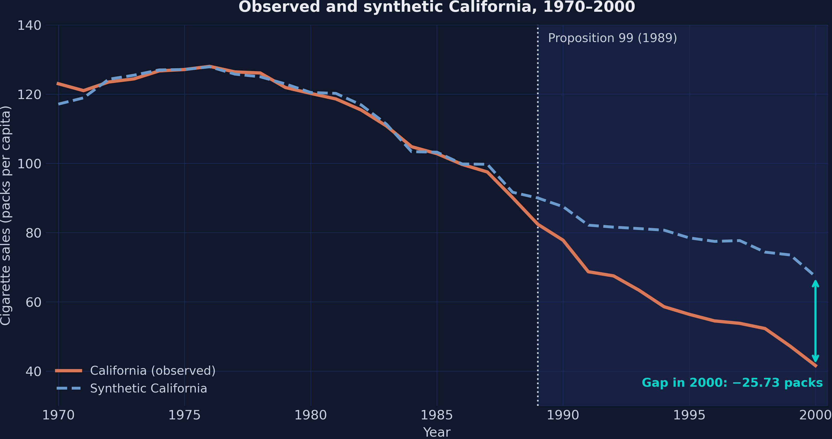
Synthetic California tracks California before 1989, with an RMSE of 1.754 packs

Observed California (orange) and its synthetic twin (dashed blue), 1970–2000; shading marks 1989–2000.

The typical miss before 1989 is 1.5 percent of mean sales, close enough for a credible counterfactual.

Before we read any effect, we check the fit before 1989. The RMSE of 1.754 packs is about 1.5 percent of mean sales of 116.21 packs over 1970–1988. The R² of 0.976 says that the synthetic path reproduces almost all the variation of sales before the program. The largest miss, 5.90 packs, occurs in 1970 at the start of the series, and later misses are much smaller. Stata reports an RMSE of 1.756 and an R² of 0.974, and the gap in the R² comes from another definition.

By 2000, California sold 38 percent fewer packs than its synthetic twin

−38.2%

In 2000: 41.6 packs per capita in California against 67.33 in synthetic California, a gap of −25.73 packs

This is the headline number of Act II. In 2000, California sold 41.6 packs per capita, while synthetic California predicts 67.33 packs. The gap of −25.73 packs equals 38.2 percent of synthetic sales. The effect therefore grew over time instead of fading, although Act III qualifies the last two years.

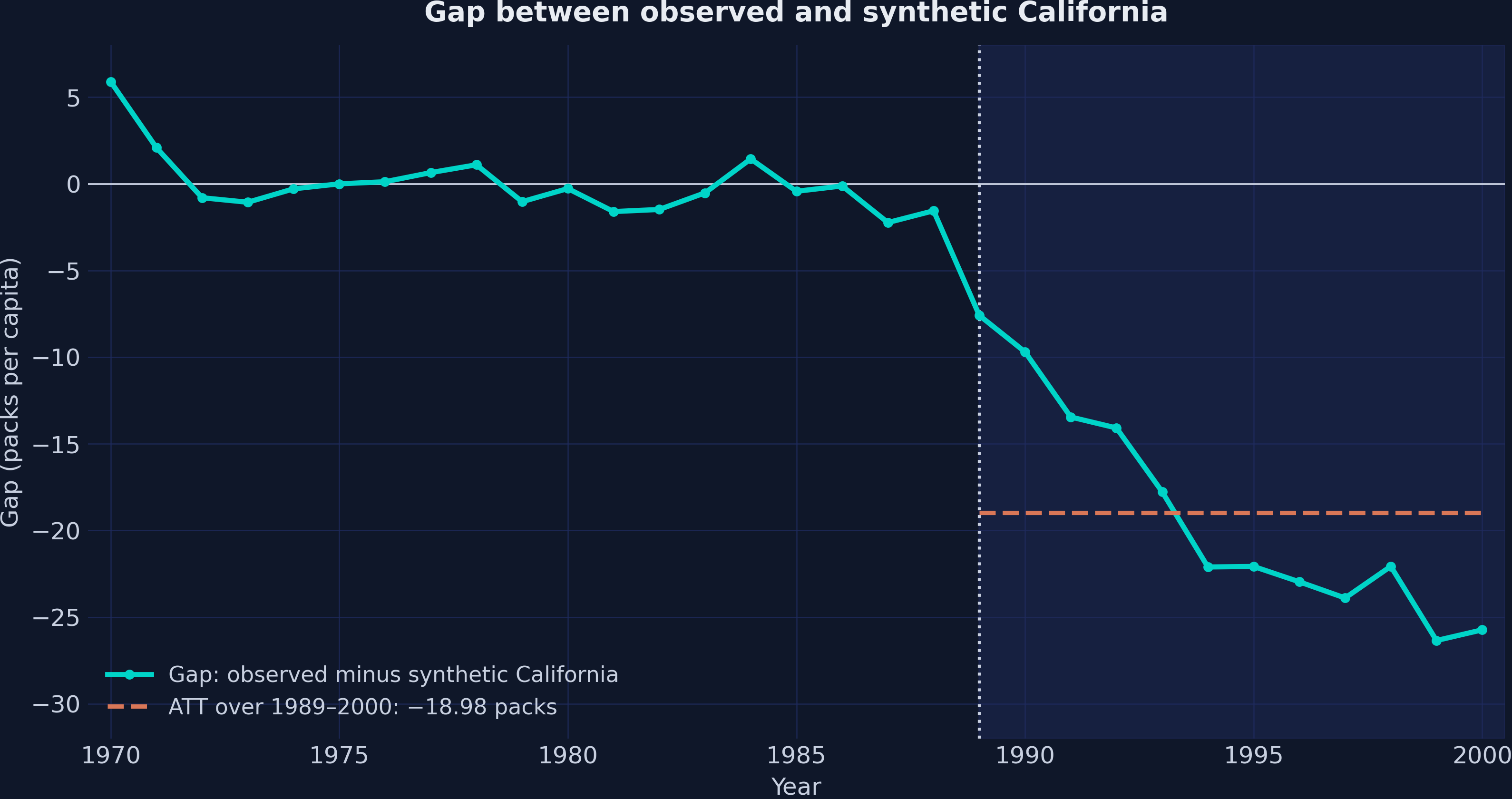
The gap widens through the 1990s, for an ATT of −18.98 packs per capita

Yearly gap between observed and synthetic California, with the ATT over 1989–2000 as a dashed orange line.

On average, California sold 18.98 fewer packs per capita per year than its twin, a reduction of 23.9 percent.

From 1971 to 1988, the gap stays small, and its largest miss is −2.23 packs, in 1987. It then drops from −1.55 packs in 1988 to −7.59 in 1989 and widens to −25.73 in 2000. The ATT averages the 12 yearly gaps: −18.98 packs per capita per year, or 23.9 percent of mean synthetic sales. Stata reports −19.00, and its rounded weights reproduce that value exactly. A gap that opens when the program starts is the visual signature of a policy effect, so Act III asks how unusual this gap is.

The Resolution

Act III

Act III tries to break the result. An average gap of 19 packs needs a yardstick, because no synthetic control predicts perfectly. We therefore measure gaps in states without the program, at a date without the program, and without each key donor.

Before you look: which states rank just below California?

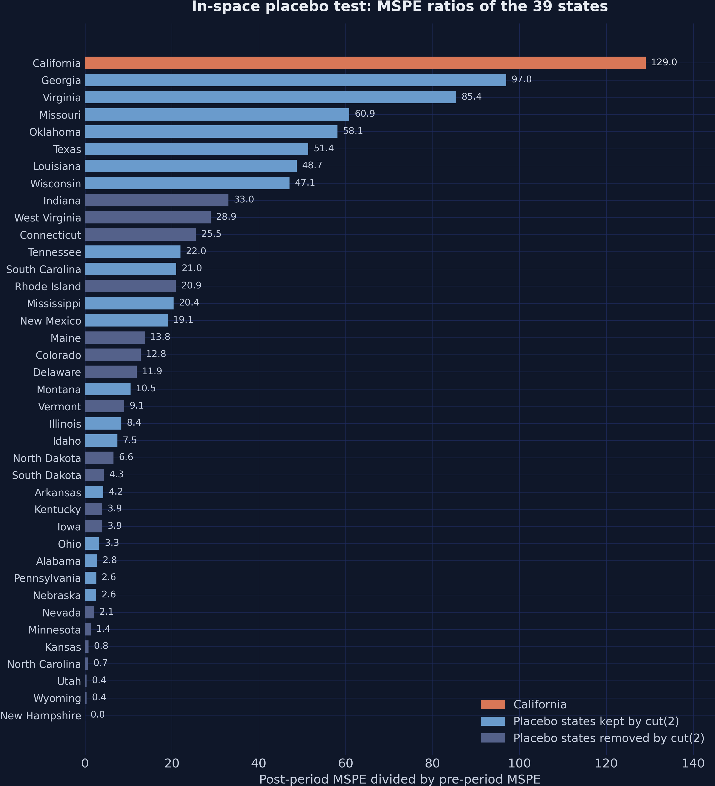
Each state takes a turn as the treated state. California has the largest MSPE ratio: its misses after 1989 are large relative to its misses before 1989. Which states rank just below it?

A.  Badly fitted states, whose large early misses inflate their ratios

B.  The donors of synthetic California, led by Utah

C.  Well-fitted states, such as Georgia and Virginia

Ask the room what a large ratio requires before 1989. Give the room 20 seconds, and then take the vote. Answer on the next slide: C. Georgia, Virginia, and Missouri rank second to fourth, and all three fit better than California before 1989. A poor fit inflates the denominator of the ratio, so badly fitted states rarely rank near the top. (AhaSlides interactive follows.)

California has the largest MSPE ratio of all 39 states, so \(p = 1/39 = 0.026\)

\[r_j = \frac{\mathrm{MSPE}_j^{\,\mathrm{post}}}{\mathrm{MSPE}_j^{\,\mathrm{pre}}}\]

Rank	State	MSPE before 1989	Ratio
1	California	3.08	129.04
2	Georgia	1.41	96.96
3	Virginia	2.74	85.42
4	Missouri	1.09	60.86

California is the most extreme of the 39 states, and 0.026 is the smallest p-value that 39 states allow.

The answer to the vote: C. Georgia, Virginia, and Missouri rank second to fourth, and each fits better than California before 1989. Their pre-treatment MSPEs are 1.41, 2.74, and 1.09, against 3.08 for California. The ratio rewards a close fit before 1989 and a large gap afterward, so a badly fitted state has a large denominator and a small ratio. The p-value is the share of the 39 states whose ratio is at least as large as that of California. California always counts itself, so rank 1 of 39 gives p = 1/39 = 0.026.

The built-in test of mlsynth reaches the same verdict. It ranks the square root of the ratio, 11.36 for California, and reports rank 1 of 39 with p = 0.026. Its placebo fits leave California out of every donor pool, while our loop keeps California in, as synth2 does.

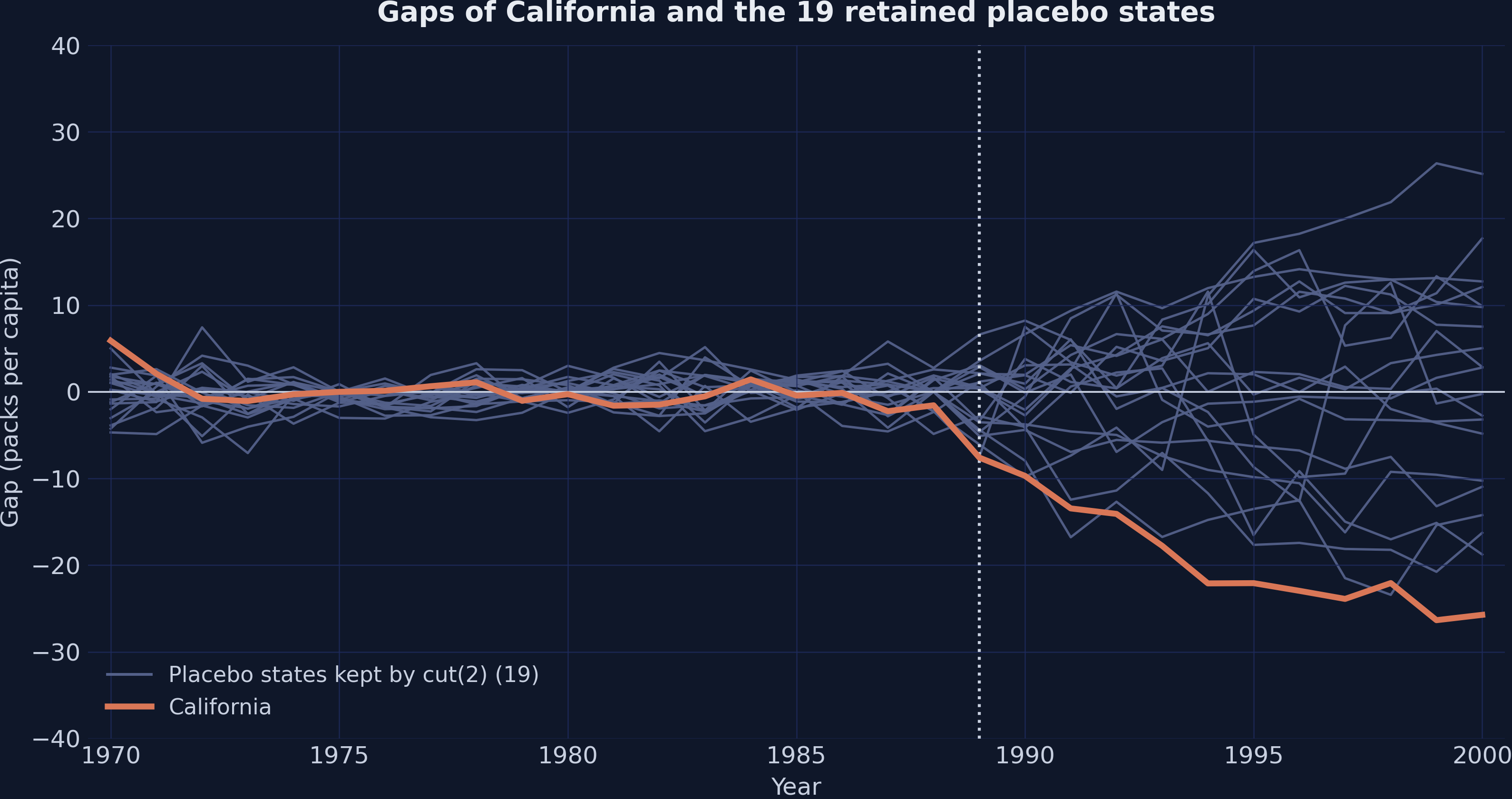
The cut(2) filter keeps 20 states, and California still ranks first: \(p = 0.050\)

Gaps of California (orange) and the 19 placebo states that cut(2) retains (gray), 1970–2000.

The filter buys comparable gaps at a price: the floor of the p-value rises from 0.026 to 0.050.

The option cut(2) of synth2 drops every placebo whose pre-treatment MSPE exceeds twice that of California, which is 3.08. It removes 19 states, including Utah and New Hampshire, whose extreme sales no weighted average can reach. It also removes Rhode Island, whose pre-treatment MSPE is about 20 times that of California. California still ranks first among the 20 states that remain, so p = 1/20 = 0.050. After 1989, its gap lies below every retained placebo in 9 of the 12 years and ends at −25.73 packs, against −18.77 for Georgia.

The cutoff is a convention, and one state sits close to it. South Dakota is removed at 2.026 times the pre-treatment MSPE of California, while Illinois is kept at 1.867. Another seed or software stack could therefore keep 21 states and change the p-value to 1/21.

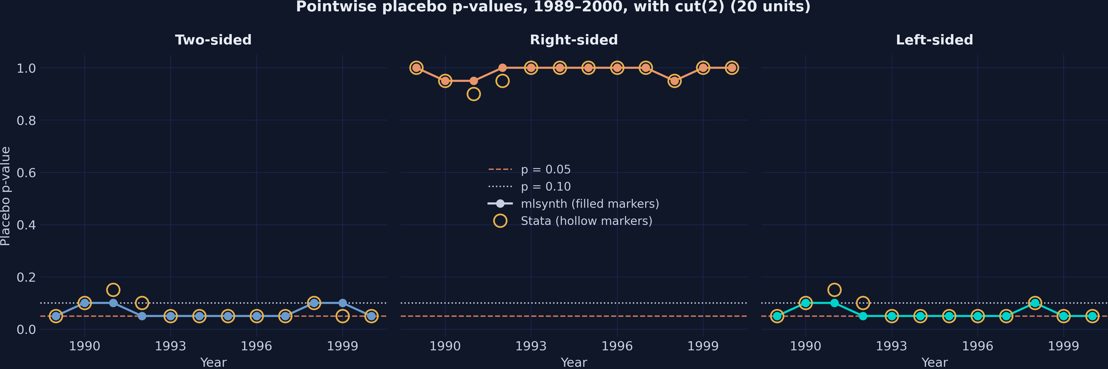
Year by year, the left-sided p-value sits at its floor of 0.050 in 9 of 12 years

Pointwise placebo p-values with cut(2), 1989–2000; filled markers show mlsynth, and hollow gold markers show Stata.

For a program designed to cut sales, the left-sided test is the relevant one, and it never exceeds 0.100.

The pointwise test repeats the ranking in each year, using the gaps instead of the ratio. Proposition 99 was designed to lower sales, so the left-sided p-value is the relevant one. It sits at its floor of 1/20 = 0.050 in 9 of the 12 years and never exceeds 0.100. Only in 1999 does the two-sided p-value exceed the left-sided one. The reason is Oklahoma, whose positive gap of 26.37 packs is larger in absolute value than the gap of California. Stata differs only in 1991, 1992, and 1999, by one step of 0.050, and its left-sided value reaches the floor in 8 of the 12 years.

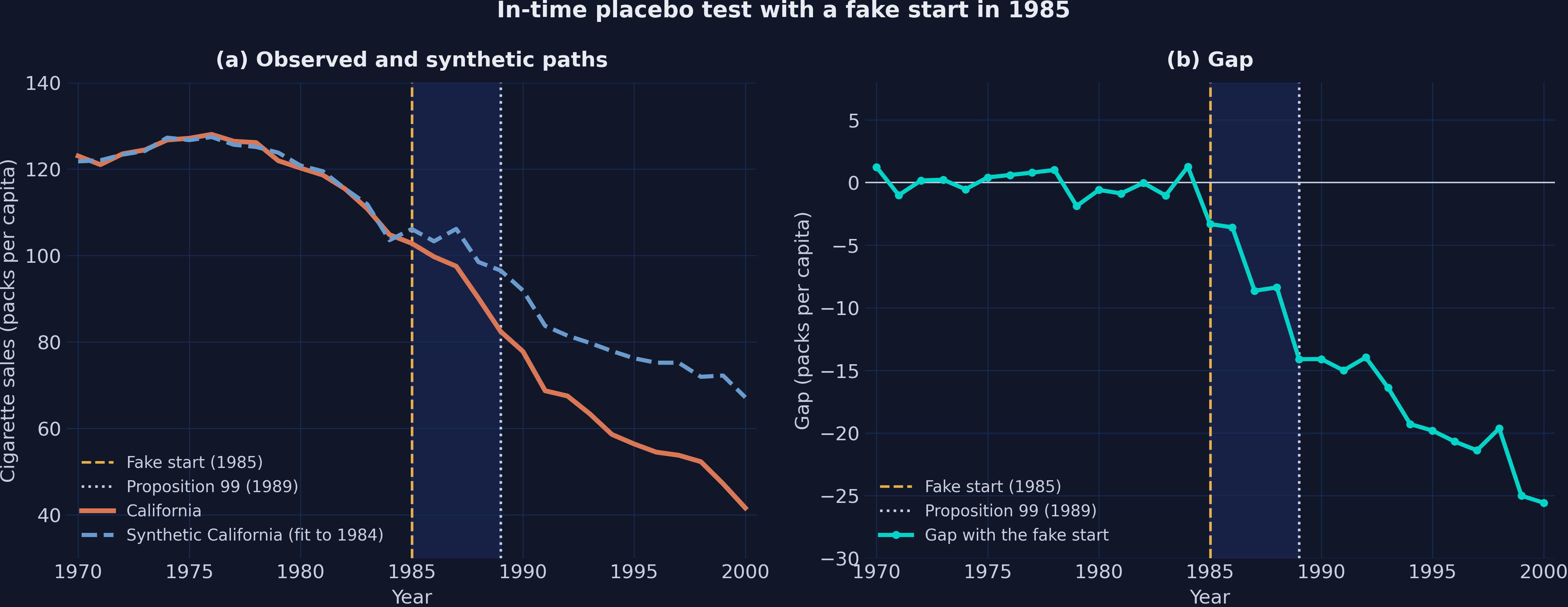
A fake start in 1985 yields gaps about one third the size of the real effect

In-time placebo with a fake start in 1985: (a) observed and synthetic paths; (b) the gap, with lines at 1985 and 1989.

The in-time test supports the timing of the effect only in part.

The in-time placebo pretends that the program began in 1985, so the model is fitted to 1970–1984. The fit is close, with an RMSE of 0.907, and the recipe uses Utah (0.351), Connecticut (0.348), and Nevada (0.301). The fake gaps for 1985–1988 range from −3.31 to −8.64 packs and average −5.97, or 0.31 times the baseline ATT. The gap then steps down by 5.74 packs, to −14.11 in 1989, and it averages −18.75 over 1989–2000. Steps of similar size already occur in 1985 and 1987, so prediction error or other changes in California may explain part of the gap.

A fake start in 1984 is not feasible. The beer data begin in 1984, so the beer average over 1980–1983 is undefined, and mlsynth stops with an MlsynthDataError. The earliest feasible fake date is therefore 1985, the date of the Stata edition.

Before you look: drop Utah and refit; which state takes over?

Utah supplies one third of synthetic California. Remove it, refit the model with the remaining 37 donors, and compare the result with the baseline.

A.  New Mexico takes over, the fit worsens, and the ATT stays near the baseline

B.  Nevada takes over, the fit improves, and the ATT doubles

C.  No state can replace Utah, and the ATT turns positive

Ask the room which state can play the role of Utah. Give the room 20 seconds, and then take the vote. Answer on the next slide: A. New Mexico, which has zero weight in the baseline, becomes the leading donor with 0.614. The pre-treatment RMSE worsens from 1.754 to 2.584, yet the ATT stays close to the baseline, at −17.52 packs. (AhaSlides interactive follows.)

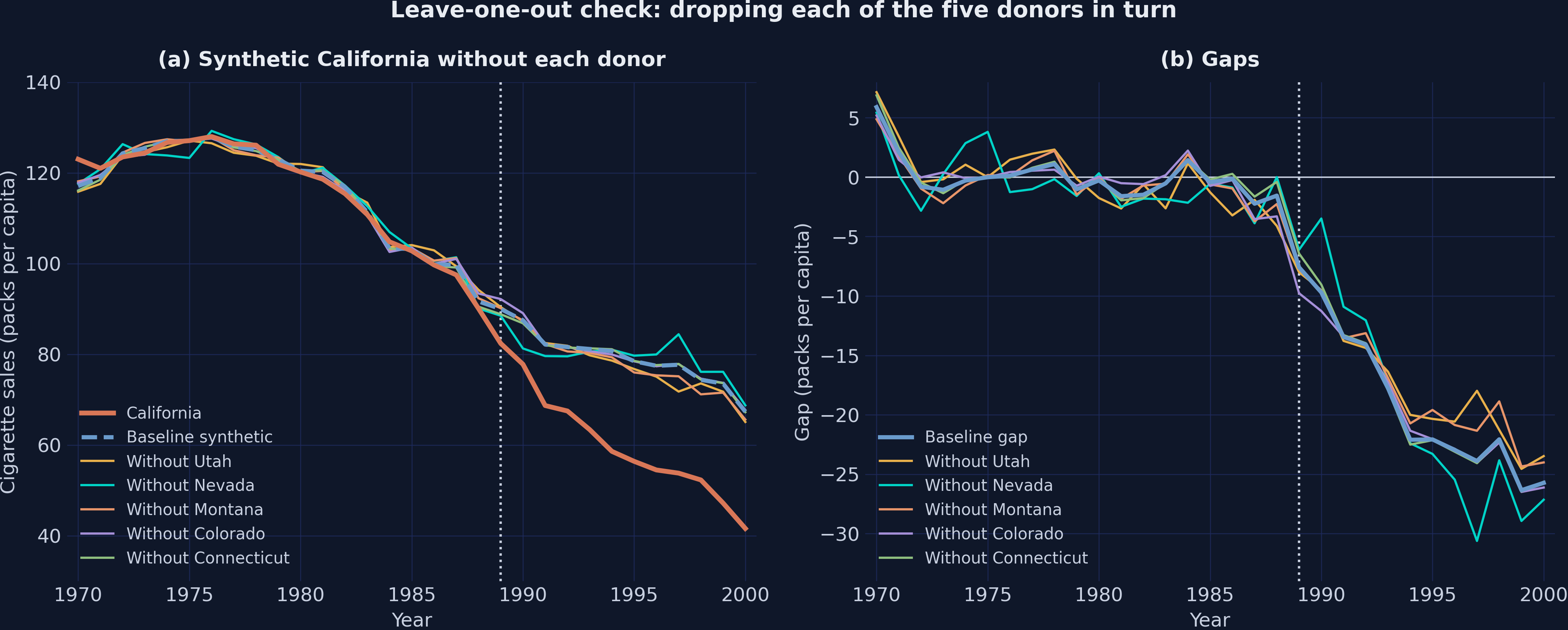
Dropping any one donor keeps the ATT between −19.29 and −17.52 packs

Leave-one-out refits that drop each of the five donors in turn: (a) synthetic paths; (b) gaps.

No single donor drives the result: every refit keeps a large, negative gap after 1988.

The answer to the vote: A. Without Utah, New Mexico takes over with a weight of 0.614, and Montana drops out. The ATT is −17.52, the smallest reduction of the five refits. Across the five refits, the ATT stays between −19.29, without Nevada, and −17.52, without Utah. Every refit lies within 1.46 packs of the baseline of −18.98. The gap in 2000 stays between −27.15 and −23.48 packs in every refit.

The refit without Nevada also speaks to spillovers. If residents of California bought cigarettes in Nevada, dropping Nevada should shrink the estimated reduction, yet it grows slightly, to −19.29. That refit, however, shifts 0.185 of the weight to New Hampshire, whose sales rose sharply after 1992, so the check cannot rule out spillovers.

Python reproduces the Stata benchmark at every step that matters

Quantity	Stata synth2	mlsynth VanillaSC	Agreement
Donor weights, Utah to Connecticut	0.334 to 0.068	0.335 to 0.068	Within 0.002
Pre-treatment RMSE	1.756	1.754	Close
ATT, packs per capita per year	−19.00	−18.98	Exact with the Stata weights
Placebo rank and p-value	1 of 39; 0.026	1 of 39; 0.026	Exact
States kept by cut(2) and p-value	20; 0.050	20; 0.050	Exact, the same 20 states
\(V\) on age share, price, and sales in 1975	0.546, 0.017, 0.422	0.332, 0.334, 0.334	Different: \(V\) is not identified

Every remaining difference has a documented source: the optimizer, rounding, a non-identified \(V\), or a definition.

The scorecard compares each step with the Stata log. The donor weights differ by less than 0.002, because the two optimizers stop at slightly different points of a flat objective. Stata rounds its weights to three decimals before it predicts, and those rounded weights reproduce its ATT of −19.0018 by hand. The placebo rank, the p-value, and the 20 states kept by cut(2) agree exactly. The predictor weights differ sharply, but V is not identified, so this difference needs no reconciliation.

Two further differences have simple sources. The R² differs because synth2 divides by the variation of synthetic California, and with that definition Python also gives 0.974. The MSPE ratio of California is 123.5 in Stata against 129.0 in Python, because the Stata placebo command refits California with a weaker search.

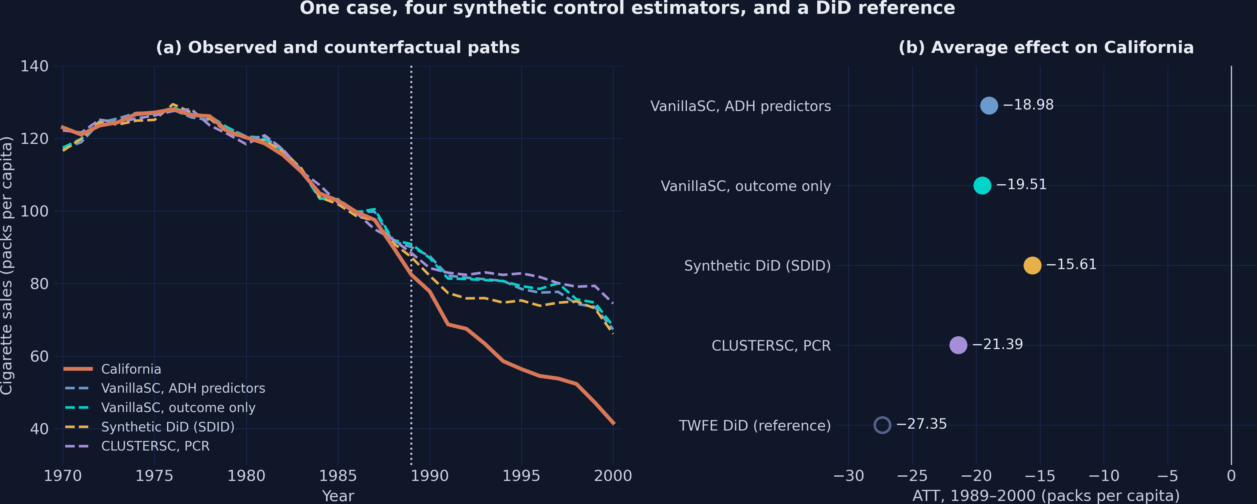
Four mlsynth estimators, one sign: the ATT ranges from −15.61 to −21.39

(a) Observed California and four counterfactual paths; (b) the four ATTs and a TWFE reference at −27.35 (hollow marker).

All four estimators find a large reduction, while TWFE inherits the poor fit of the simple average.

The tour reuses the same dictionary with three other estimators. The outcome-only fit matches the 19 pre-treatment outcomes directly and gives −19.51 with six donors. Synthetic difference-in-differences adds time weights and a level shift and gives −15.61. CLUSTERSC with principal component regression gives −21.39 with 34 donors, 11 of them with negative weights, and −19.37 when its clustering step is switched off. The TWFE reference of −27.35 weights all 38 donors equally, so it inherits the poor match of the simple average before 1989.

The gap was already large before Proposition 10 raised the tax again in 1999

Objection. The gap of 38.2 percent in 2000 measures Proposition 99 alone.

Response. In January 1999, Proposition 10 added 50 cents per pack, so the gaps of 1999 and 2000 mix two programs. Yet the gap stayed below −22 packs in every year from 1994 to 1998.

The growth of the effect does not rest on the last two years.

We steelman the objection first, because the largest gaps arrive in 1999 and 2000. Proposition 10 raised the state cigarette tax by a further 50 cents per pack in January 1999. The gaps of those two years therefore cannot be credited to Proposition 99 alone, and the same caveat applies to the headline of 38.2 percent in 2000. Even before that second increase, however, the gap stayed below −22 packs in every year from 1994 to 1998. The large and persistent effect thus does not depend on the last two years.

Five tempting misreadings

Common misconceptions

Synthetic control results are easy to state and easy to misread. Each of the next five slides states a tempting claim about this analysis. Each slide then answers the claim with the numbers of this tutorial.

“Synthetic California is built from its neighbors”: only Nevada borders it

Myth. Synthetic California blends the neighbors of California.

Truth. Of the five donors, only Nevada borders California. Utah (0.335), Montana (0.202), Colorado (0.160), and Connecticut (0.068) enter because their weighted combination tracks sales before 1989.

The recipe is chosen for its fit, not for its geography.

Arizona and Oregon, the other neighbors of California, are absent from the data, because they ran their own large tobacco programs. A donor need not resemble California on its own. Utah, the largest donor, sold 55.0 packs in 1988 against 90.1 in California. The weights are chosen so that the combination tracks California before 1989 and matches most of its predictors.

“\(p = 0.026\) is the probability of no effect”: it is a rank, not a probability

Myth. A p-value of 0.026 means a 2.6 percent chance that Proposition 99 had no effect.

Truth. The p-value is the share of states whose MSPE ratio is at least as large as that of California. It cannot fall below \(1/39 = 0.026\), and it equals \(1/20 = 0.050\) after cut(2).

The p-value describes a rank in a placebo distribution, not the probability of a hypothesis.

This misreading is common in applied work. Suppose that the program had no effect in any state and that every state were equally likely to be the treated one. Each state would then be equally likely to have the largest ratio. California would then hold the top rank with probability 1/39, which is exactly the p-value. The p-value is thus a statement about the data under the null, not about the truth of the null.

“A sound in-time placebo shows zero gaps”: the standard is small gaps and no break

Myth. A valid in-time placebo must show fake gaps of exactly zero.

Truth. Prediction errors grow beyond the fitting period, so fake gaps are rarely zero. The standard is small fake gaps and no break at the fake date. Here the fake gaps average −5.97 packs, about one third of the −18.75 after 1989, and the gap already steps down in 1985.

By this standard, the in-time test of this tutorial passes only in part.

The in-time placebo is the weak spot of the analysis. Its fake gaps need not be zero, so their size alone is not the problem. The problem is the step at the fake date, which shows that California was already pulling away from its synthetic twin before 1989.

“The smallest pre-treatment error wins”: a close fit is necessary, not sufficient

Myth. The estimator with the lowest pre-treatment RMSE is the most credible.

Truth. CLUSTERSC has the lowest RMSE, 1.503, but 11 of its 34 donors carry negative weights, which extrapolate beyond the donors. The outcome-only fit beats the baseline by construction (1.656 against 1.754), yet its placebo test ranks California only third, with \(p = 0.077\).

A close fit is necessary for credibility, but it does not certify the counterfactual.

Fit before 1989 is a necessary condition, not a ranking device. Negative weights let a counterfactual leave the range of the donors, which the simplex constraint of the baseline forbids. The weaker placebo test of the outcome-only fit shows that a closer fit need not yield stronger evidence.

“cut(2) can only strengthen the evidence”: it trades resolution for comparability

Myth. Dropping badly fitted placebos with cut(2) can only strengthen the evidence.

Truth. The filter shrinks the comparison set from 39 to 20 states, so the smallest attainable p-value rises from 0.026 to 0.050. With a cutoff of 1, only 9 states remain, and the p-value cannot fall below 0.111, although California still ranks first.

The filter buys comparability of the gaps at the cost of resolution.

A badly fitted state has a large pre-treatment MSPE, so its ratio tends to be small already, and the filter seldom helps California climb the ranking. What the filter buys is comparability of the gaps themselves, which matters for the gap figure and the pointwise test. What it costs is resolution, because every p-value then moves on a coarser grid.

A synthetic twin earns trust by fitting the past and keeps it only by surviving attempts to break it.

This sentence is the single takeaway of the talk. Synthetic California earned trust with a close fit from 1970 to 1988, and it kept that trust through the placebo test, the leave-one-out refits, and the estimator tour. The fake start in 1985 passed only in part, so the timing of the onset remains less certain than the size of the effect. Our answer to the question is a reduction of 18.98 packs per capita per year over 1989–2000, or 23.9 percent.