Introduction to Panel Data Methods

Seven estimators, one wage panel: why the union premium triples

0.075pooled OLS — cross-sectional

0.210fixed effects — within-worker

73of 2,199 workers switch status

Carlos Mendez

Nagoya University (GSID)

October 2, 2026

The Tension

Act I

Same workers, same question — but the answer triples depending on the estimator

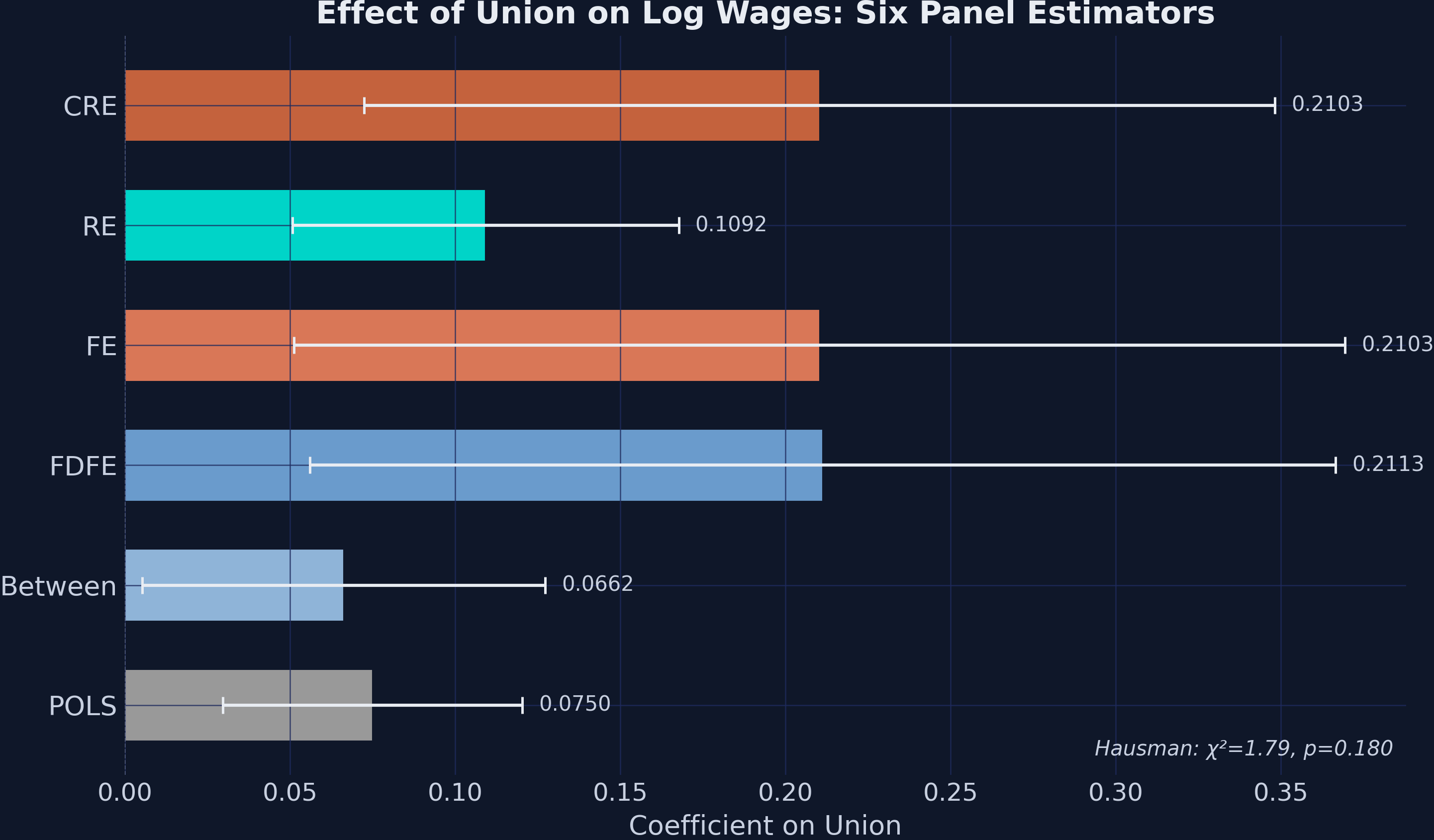
A simple regression says joining a union raises wages by 7.5 log points. Compare each worker to themselves across years and the number jumps to 21 log points (about 23%).

One dataset, two stories. Which one do you report?

The central tension of the tutorial: pooled OLS and the within (fixed-effects) estimator answer the same applied question — what does union membership do to wages — but disagree by a factor of three. The gap is not noise; it is the empirical signature of selection on unobservables. Everything in Act II is about earning the right to pick a number.

Six estimators on one panel disagree by a factor of three

Six panel estimators with 95% CIs. POLS / Between / RE cluster near 0.07–0.11; FDFE / FE / CRE cluster near 0.21. The classical Hausman test is annotated.

The spoiler figure. Don’t explain every bar yet — just plant that the estimators split into two camps roughly three-fold apart, and that we come back to this picture in Act III. Cross-sectional methods (POLS 0.075, Between 0.066, RE 0.109) on one side; within methods (FDFE 0.211, FE 0.210, CRE 0.210) on the other.

Where we’re going

• The data: a balanced 2-period, 2,199-worker wage panel
• Between vs within variation — what each estimator can actually use
• Seven estimators, escalating discipline: POLS → Between → FD → FE → TWFE → RE → CRE
• Hausman and Mundlak — choosing between fixed and random effects

Teaching deck, so we signpost. Seven “Before you look” slides along the way ask the room to predict before each reveal; on AhaSlides each one is followed by a live quiz.

The Investigation

Act II

The lab: 2,199 workers, two years, a perfectly balanced T = 2 panel

• Outcome — log hourly wage (\(\bar y = 3.11\), SD 0.60)
• Treatment — union membership; only 16.3% of worker-years unionized
• Window — restricted to 2010 and 2012, so \(T = 2\) and the panel is balanced

With \(T = 2\), every worker contributes exactly two rows — the cleanest setting to see that first differences and the within estimator are exactly linked: FD without an intercept is FE, and FD with an intercept is two-way FE.

NLSY-style data on US workers; the full file has five waves (2010–2018) but we keep two for pedagogical clarity. 4,398 worker-year observations, balanced. The low unionization rate (16.3%) matters: any estimator that leans on cross-sectional variation is working mostly with non-union workers.

Each estimator chooses which variation to believe

Cross-sectional camp

• POLS — ignores the panel
• Between — worker means only
• RE — GLS-weighted blend

Answers: “union vs non-union workers?”

Within camp

• FD / FDFE — period differences
• FE / TWFE — demeaned data
• CRE / Mundlak — the bridge

Answers: “same worker, switched status?”

Hausman and the Mundlak term are the formal tests for choosing between the two camps.

This columns slide replaces the post’s Mermaid decision diagram (Quarto revealjs does not bundle mermaid.js, so a fenced mermaid block would render as raw text). The left side leans on between-worker variation; the right side on within-worker variation. CRE/Mundlak sits in the middle and recovers both. We will run both specification tests, and they disagree: the reason (which errors each test assumes) is part of the lesson.

Before you look: how much of union’s variance is within workers?

Union status has an overall SD of 0.369 and a mean of 16.3%. What share of its variance comes from workers who change status between 2010 and 2012?

A.  Less than 10%

B.  About 25%

C.  About 50%

Ask the room to commit before the decomposition. Give 20 seconds, then take the vote. Answer on the next slide: A, only 6.1% is within. The within SD (0.0911) is not a share; the share is its square over the sum of the squared between and within SDs. Just 73 of 2,199 workers switch. (AhaSlides interactive I1 follows.)

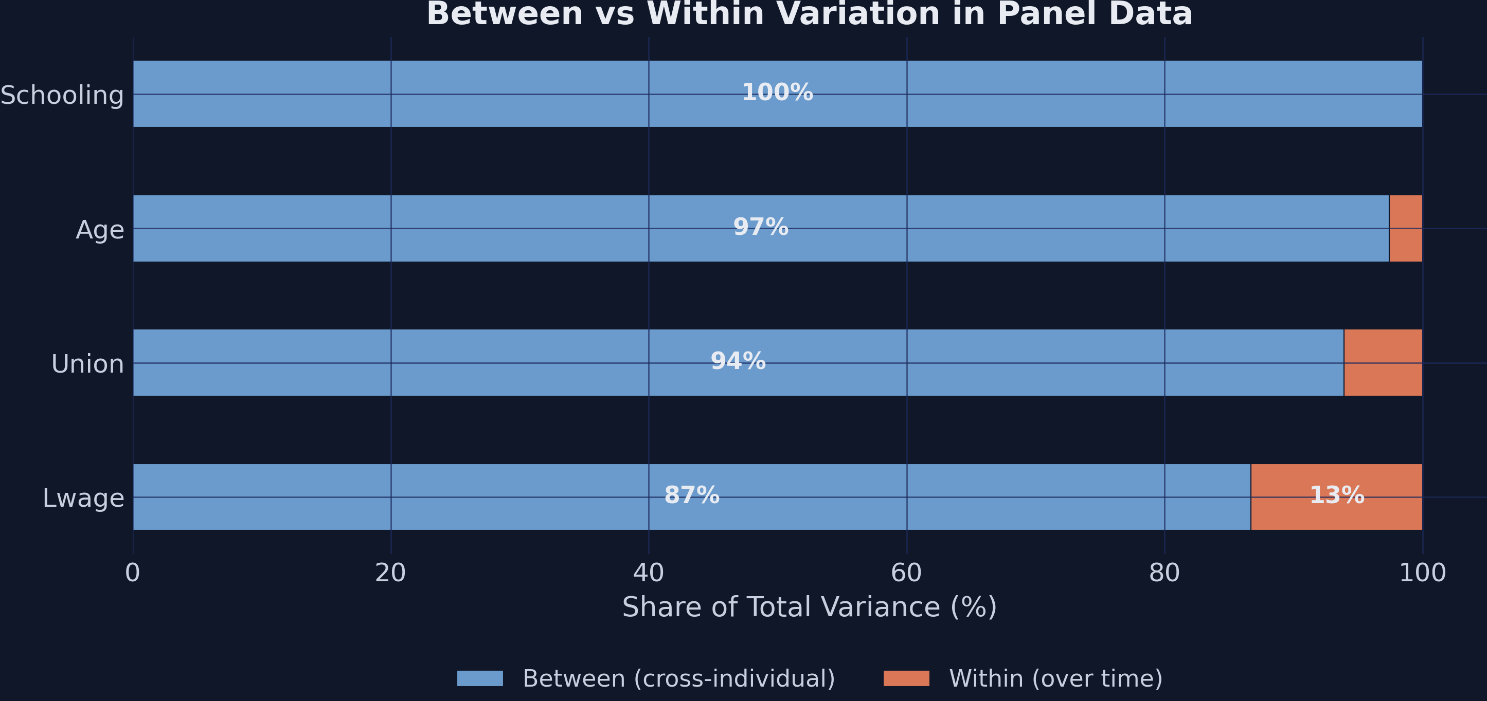
94% of union variation is between workers — only 6.1% is within

Between vs within variance shares for the four key variables. Union is 93.9% between; schooling is 100% between (zero within).

The answer to the vote: A. Fixed effects only use the within part. For union that is a thin 6.1% slice of total variance. Schooling has zero within-variation (nobody’s education changes across two years), so FE mechanically drops it. The consequence: FE standard errors will be much larger than POLS — the FE-vs-RE choice is about precision as much as bias.

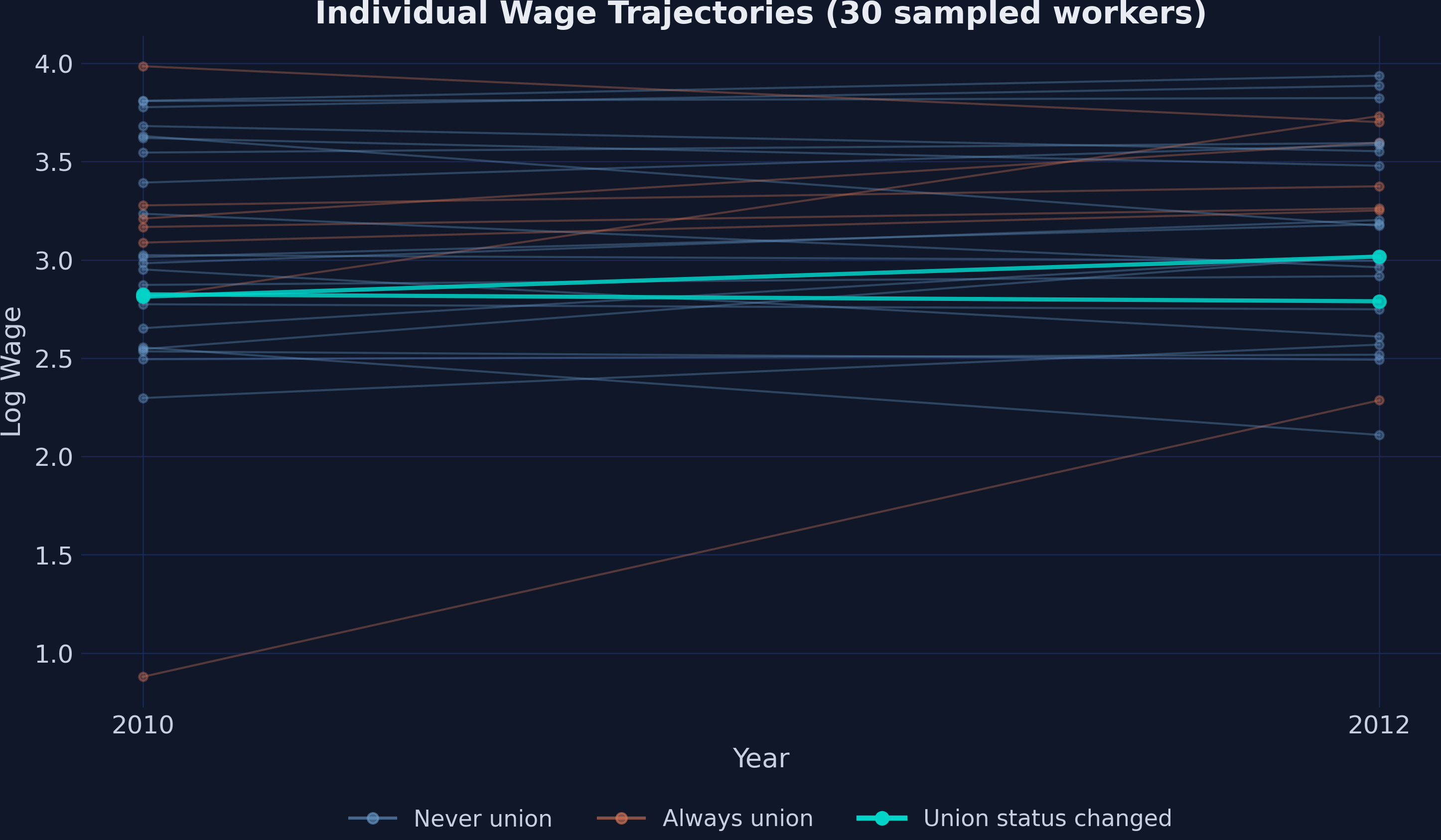
Only the workers who switch status identify the within estimators

Log-wage trajectories for 30 sampled workers. Teal lines change union status; orange/blue lines never do.

Most lines are flat-colored — always-union (orange) or never-union (blue). Only the teal “changer” lines carry identifying information for FE, FD, and Mundlak. One-way fixed effects reads only the teal lines, because a line whose union status never changes carries no within-worker contrast; the blue and orange lines can only be compared with each other, which is the cross-sectional comparison. The tension is literally a question of which lines you choose to read.

Pooled OLS — the naive baseline — reports a 7.5-log-point premium

fit_pols = pf.feols("lwage ~ union", data=df, vcov="HC1")
print(fit_pols.coef()["union"])   # 0.0750
# Union coefficient: 0.0750  (SE 0.0231)

Highly significant (\(t \approx 3.25\)) — and almost certainly biased if ability selects out of union jobs.

POLS treats every worker-year as independent, ignoring the panel. 7.5 log points, SE 2.3. This is the textbook cross-sectional answer and the number a naive analyst reports. The rest of the post is a tour through ways of subtracting the selection bias out. Between is its near-twin (0.066) because 94% of union variance is between-worker.

Before you look: smaller, the same, or larger than pooled OLS?

Pooled OLS gave 0.0750 (SE 0.0231). Now subtract each worker’s 2010 values from the 2012 values and regress the change in log wage on the change in union status.

A.  Smaller than 0.075

B.  About the same

C.  Larger, with a larger standard error

Ask: which way does first-differencing move the estimate, and what happens to its precision? Answer on the next slide: C. FD gives 0.2113 with SE 0.0792, about 3.4 times the POLS SE: differencing removes the fixed traits that depress the cross-sectional comparison but keeps only the 73 switchers. (AhaSlides interactive I2 follows.)

First-differencing erases \(\alpha_i\) and triples the estimate to 0.211

\[y_{i,2012} - y_{i,2010} = \beta\,(x_{i,2012} - x_{i,2010}) + (u_{i,2012} - u_{i,2010})\]

The worker-specific effect \(\alpha_i\) — ability, schooling, gender — cancels in the subtraction. What is left is identified only by workers who changed union status.

FDFE \(= 0.2113\) (SE 0.079); the SE is \(3.4\times\) larger than POLS — the switcher-only signature.

The answer to the vote: C. Start from y_it = α_i + β x_it + u_it; difference across the two periods and α_i drops out. The point estimate is almost three times POLS (0.211 vs 0.075) with a wide CI [≈0.06, 0.37] that excludes zero but also contains the POLS 0.075, so the upward revision is large in size but not statistically decisive on its own. Workers who switch into unions are a different population from always-union workers, so the within parameter is genuinely different — and arguably cleaner.

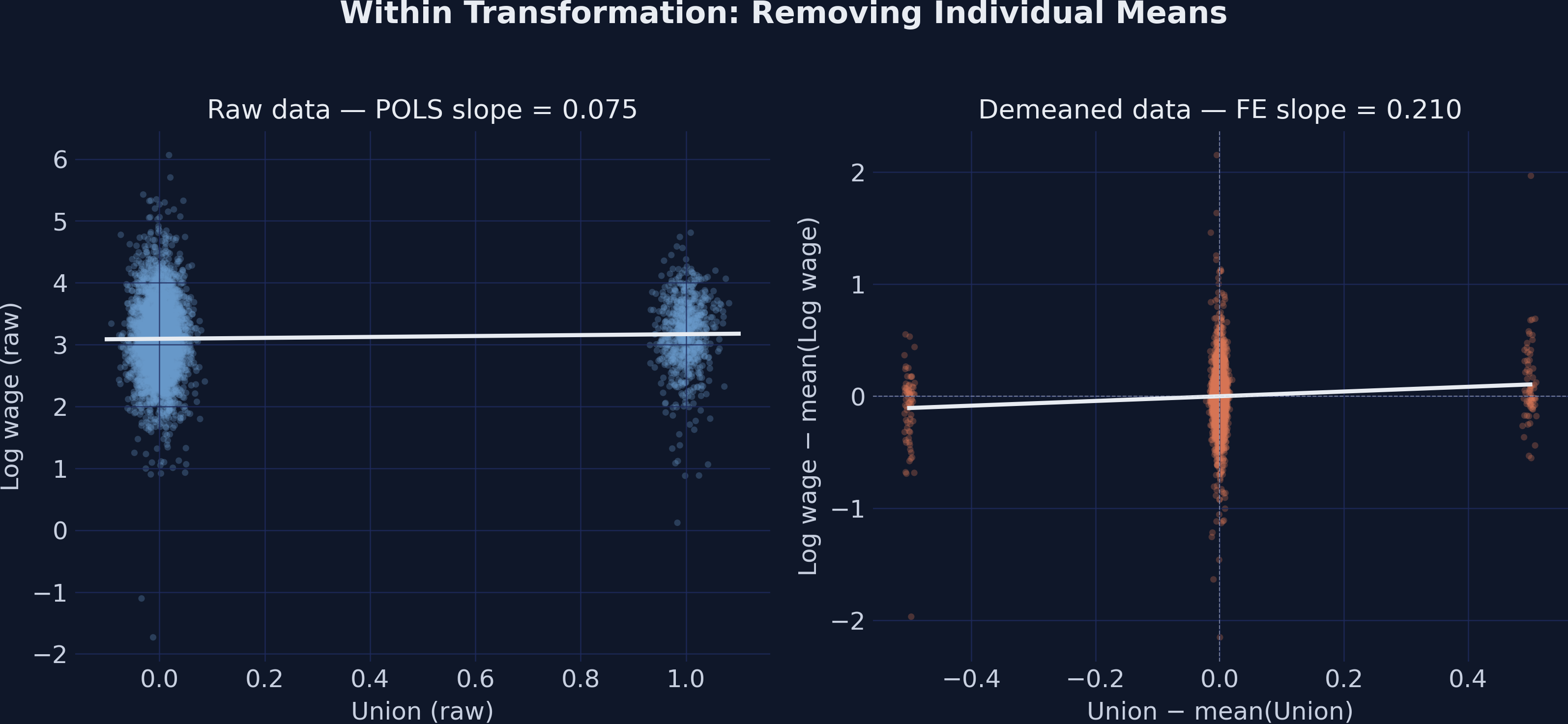
The within transformation demeans the data — and the slope steepens to 0.21

Within transformation: raw scatter with the shallow POLS slope (left); demeaned scatter with the steeper FE slope through the origin (right).

Same observations, two pictures. Left (raw): POLS slope 0.075, dragged down because union and non-union mean wages sit close together. Right (demeaned): FE slope ≈ 0.21, identified only by the points that move off the origin — the switchers. The within estimator subtracts each worker’s mean, so α_i vanishes; OLS on the demeaned data gives the FE coefficient.

Before you look: does fixed effects match FD’s 0.2113?

With only two periods, demeaning and differencing use the same 73 switchers. Will the within (FE) estimate equal the FD estimate of 0.2113?

A.  Exactly equal

B.  Slightly different

C.  Very different

Ask, and as a follow-up: if it differs, which feature of the FD regression could explain the gap? Answer on the next slide: B. FE gives 0.2103, a gap of 0.001, because the FD regression has an intercept that absorbs the common wage growth of 0.0727. Without the intercept FD returns exactly 0.2103. (AhaSlides interactive I3 follows.)

Three recipes, one number: FD, demeaning, and dummy FE all give 0.2103

fit_fe   = pf.feols("lwage ~ union | ID", data=df, vcov="HC1")        # absorbed FE
fit_dvfe = pf.feols("lwage ~ union + C(ID_str)", data=df, vcov="HC1") # 2,198 dummies
# Both → 0.2103;  FDFE → 0.2113 (the +0.001 is an intercept-driven year trend)

Within transformation, first-differences, and dummy-variable FE are three recipes for the same dish. Absorption (| ID) is just the fast one.

The answer to the vote: B, slightly different. DVFE with N−1 = 2,198 worker dummies recovers 0.2103 exactly. Modern software prefers absorption purely for speed: about 2,200 dummies still run fast, but at N = 100,000 the dummy spec is prohibitive while absorbed FE stays trivial. The FDFE +0.001 gap is the common time trend: FD without an intercept returns 0.2103, and adding a year effect to FE reproduces FD with an intercept (0.2113) — that is two-way FE, next.

Before you look: where does two-way FE land?

FE gave 0.2103 and FD gave 0.2113. Adding year effects to FE allows a common wage trend.

A.  Exactly equal to FD, 0.2113

B.  Equal to FE, 0.2103

C.  Somewhere else

Ask the room to pick before the code. Answer on the next slide: A. With T = 2 the year effect plays exactly the role of the FD intercept, so two-way FE equals FD with an intercept to six decimals. (AhaSlides interactive I4 follows.)

Two-way FE absorbs year shocks and lands at 0.2113 — exactly first differences

fit_twfe = pf.feols("lwage ~ union | ID + year", data=df, vcov={"CRV1": "ID"})
# Union coefficient: 0.2113  (SE 0.0792)

Absorbing the year effect removes the aggregate wage trend FD’s intercept was capturing. Time-invariant regressors (schooling, female) are silently absorbed.

The answer to the vote: A. TWFE = 0.2113, identical to FD with an intercept: with T = 2 the two coincide exactly, while one-way FE (0.2103) equals FD without an intercept. The 0.001 gap is the common time trend that the year effect and FD’s intercept both absorb. You cannot identify the effect of something that does not change within a worker — which is why applied researchers reach for CRE/Mundlak when they want within identification AND coefficients on time-invariant variables.

Random effects bets on no-correlation — and is pulled toward POLS at 0.109

exog = sm.add_constant(df_re[["union"]])
fit_re = RandomEffects(df_re["lwage"], exog).fit(cov_type="robust")
# Union coefficient: 0.1092  (SE 0.0299)

RE is a variance-weighted average of between and within. With only 6% within, it leans toward the between picture — and SE is \(2.7\times\) tighter than FE.

RE treats α_i as a random draw uncorrelated with the regressors and uses GLS to blend within and between efficiently. Here it lands at 0.109, squarely between POLS (0.075) and FE (0.210), leaning toward POLS because within variation is thin. The SE (0.030) is striking — but that precision is real only if individual effects are uncorrelated with union status. The FE–POLS gap suggests they are not, so the precision is bought with bias.

Before you look: what do robust SEs do to the Hausman statistic?

The textbook test uses classical SEs: 0.0509 for FE and 0.0278 for RE. The robust SEs are larger, 0.0812 and 0.0299. Plug the robust ones into the same formula, and H will…

A.  Rise, so the test rejects more strongly

B.  Fall enough to flip the verdict

C.  Fall, but still reject at 5%

Ask: the robust FE SE grows much more than the robust RE SE, so what happens to the denominator V_FE − V_RE? Answer on the next slide: B. H falls from 5.62 (p = 0.018) to 1.79 (p = 0.180). But the plug-in number is not a valid test, because with robust errors V_FE − V_RE is no longer the variance of the difference. (AhaSlides interactive I5 follows.)

The textbook Hausman test rejects RE, if the errors are classical

\[H = (\hat\beta_{\mathrm{FE}} - \hat\beta_{\mathrm{RE}})'\,[V_{\mathrm{FE}} - V_{\mathrm{RE}}]^{-1}\,(\hat\beta_{\mathrm{FE}} - \hat\beta_{\mathrm{RE}}) \sim \chi^2(k)\]

With classical variances (SE 0.0509 for FE, 0.0278 for RE): \(H = 5.62\), \(p = 0.018\), so we reject RE at 5%.

Plugging the robust SEs into the same formula gives \(H = 1.79\), \(p = 0.180\), but that is not a valid test: \(V_{\mathrm{FE}} - V_{\mathrm{RE}}\) is the variance of the difference only when RE is efficient.

The answer to the vote: B, the verdict flips, but only in an invalid test. β_FE − β_RE = +0.101. The textbook test (Stata’s hausman fe re, R’s phtest) uses classical variances because its formula relies on RE being fully efficient under the null. That gives H = 5.62 on 1 df, p = 0.018: reject. The robust SEs are much larger, especially for FE (0.0812 vs 0.0509), which suggests the classical assumption is doubtful. Plugging them in flips the verdict (H = 1.79, p = 0.180), but the result has no chi-square distribution. With robust errors, the valid check is the Mundlak test, next.

Before you look: what happens to the union coefficient in CRE?

Random effects gave 0.1092. Now add each worker’s mean union status, union_bar, as a regressor and re-estimate random effects.

A.  It equals the FE value, 0.2103

B.  It stays near 0.11

C.  It moves between 0.11 and 0.21

Ask the room to commit. Answer on the next slide: A, exactly 0.2103. Once the worker mean of union status is controlled for, the only variation left in union is within variation, so RE has nothing else to use; this holds for any RE weight θ. (AhaSlides interactive I6 follows.)

Mundlak recovers the FE coefficient and flags negative selection

\[y_{it} = \alpha + \beta\,x_{it} + \gamma\,\bar{x}_i + a_i + u_{it}\]

Add each worker’s mean union exposure \(\bar{x}_i\), then run RE (random worker effect \(a_i\)). The within coefficient \(\beta\) equals FE; the mean coefficient \(\gamma\) tests whether \(\alpha_i\) correlates with \(x\).

CRE within \(= 0.2103\) (matches FE exactly); Mundlak term \(\gamma = -0.144\), \(p = 0.072\) — borderline, hinting at negative selection.

The answer to the vote: A. Mundlak (1978) proved β here is numerically identical to FE — and it is, to four decimals (0.2103). The γ on union_bar is −0.144, p = 0.072: workers with higher average union exposure earn less even after conditioning on within changes, consistent with lower-wage workers selecting into unions. In this balanced panel γ is exactly Between minus FE (0.0662 − 0.2103). Unlike the plug-in Hausman number, this test stays valid with robust SEs; clustered by worker it gives p = 0.106. So: the textbook test rejects, the robust test is borderline.

The Resolution

Act III

Within-worker, joining a union pays 0.21 log points — nearly triple the naive 0.075

0.210

\(\hat\beta_{\mathrm{FE}}\) on union (SE 0.081) — vs pooled OLS 0.075; FDFE, TWFE, and CRE all agree near 0.21

The Act-III payoff. Cross-sectional methods say 7–11 log points; within methods say about 21. The factor-of-three gap is the empirical signature of selection on unobservables: higher-ability workers are less likely to be unionized in this sample, so cross-sectional comparisons understate the within-worker payoff to joining a union. Caveat for Q&A: the 0.21 rests on 73 switchers and is specific to 2010–2012; with all five waves two-way FE falls to 0.040 (SE 0.026).

Two camps, three-fold apart — and the gap is selection, not noise

Method	Coef	SE	Variation used
POLS	0.0750	0.0231	all (ignores panel)
Between	0.0662	0.0311	cross-sectional means
RE	0.1092	0.0299	GLS between + within
FDFE	0.2113	0.0792	within differences
FE	0.2103	0.0812	within demeaned
TWFE	0.2113	0.0792	within, net of year effects
CRE	0.2103	0.0703	RE + Mundlak (= within)

Cross-sectional 7–11 log points · within ~21. Standard errors swing inversely — the within camp is noisier but causally cleaner.

The payoff table. The seven methods cluster into two camps roughly three-fold apart; TWFE equals FDFE exactly because T = 2. Cross-sectional standard errors are 2.6–3.5× smaller, but these methods identify a biased (under our hypothesis) parameter; within methods are noisier but cleaner under weaker assumptions. Reporting both estimands side by side is more honest than picking one.

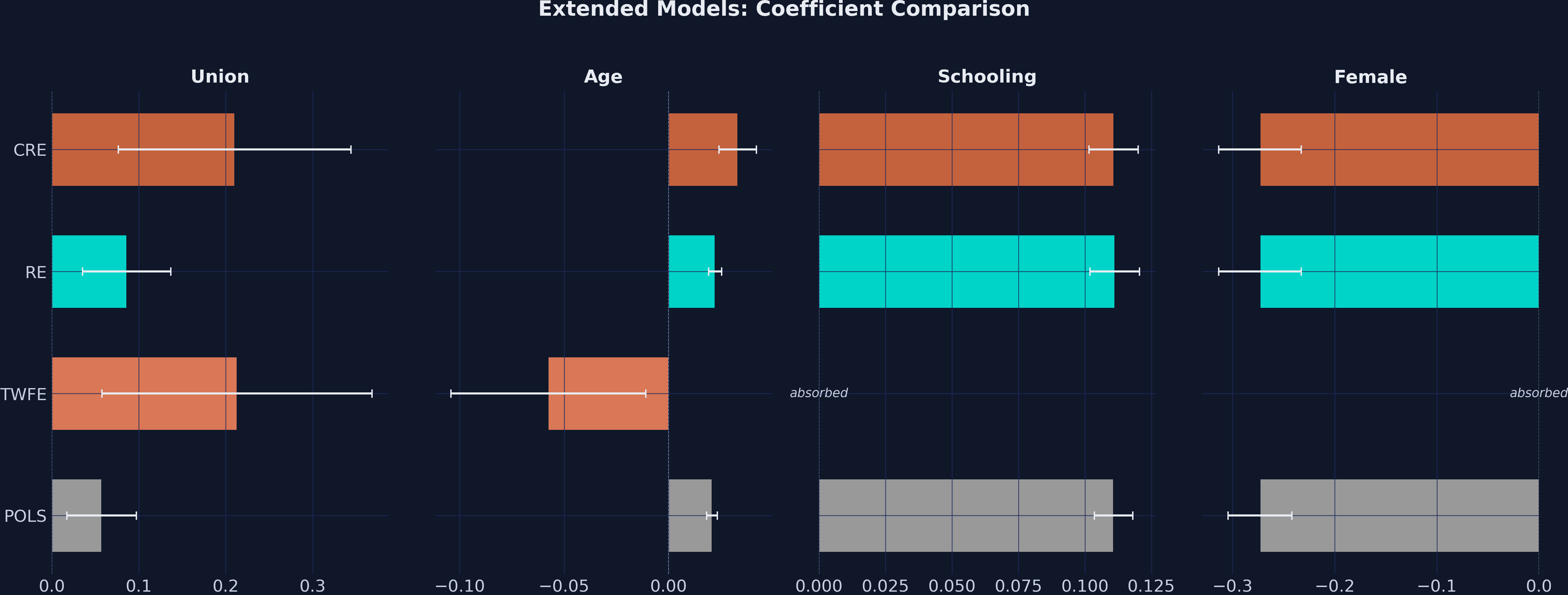
Before you look: what happens to the age coefficient under two-way FE?

With controls, each extra year of age raises log wages by about 0.02 in pooled OLS. Two-way FE absorbs both worker and year effects. Under two-way FE, the age coefficient will…

A.  Stay near +0.02

B.  Change sign

C.  Shrink toward zero

Ask, then hint: between 2010 and 2012 most workers age by exactly two years. Answer on the next slide: B, it turns negative (−0.0576). The year effect absorbs the two-year step for 1,885 workers, so the coefficient rests on the 314 whose interviews were not exactly two years apart: fragile, not an age profile. (AhaSlides interactive I7 follows.)

Adding controls leaves the two-camp gap intact

Extended models — union, age, schooling, female across POLS / TWFE / RE / CRE. The within premium survives controls.

The answer to the vote: B, the within age coefficient turns negative. With age, schooling, female, and year effects in every model, POLS drops to 0.057 (controls absorb some confounding) and RE to 0.088, but TWFE and CRE both report 0.213; CRE reproduces the TWFE coefficients exactly. Schooling (+11.1 log pts/yr) and the female penalty (−27.3 log pts) are stable across POLS/RE/CRE because they are time-invariant — and absorbed by FE. The within age coefficient (TWFE and CRE) flips to −0.058, a fragile estimate (age is not exactly collinear with the year dummy, but only the 314 workers whose age did not rise by exactly two years identify it), not a real age–wage relationship.

Does FE make this causal? No — strict exogeneity still carries the weight

Objection. Within estimators just net out fixed traits — they can’t manufacture identification.

Response. Correct. FE/FDFE/TWFE/CRE target the average effect among union switchers only — and only under strict exogeneity given the worker fixed effect.

Steelman, don’t strawman. They remove time-invariant confounders, not time-varying ones — a promotion that coincides with joining a union still biases the within estimate. POLS and Between carry no causal reading absent unconfoundedness. Fixed effects discipline the comparison; they do not relax identification. The within estimand is local — it is identified off the 73 of 2,199 workers (3.3%) who switched union status (36 joined, 37 left) — and rests on strict exogeneity conditional on α_i. Reporting both the within and cross-sectional estimands, as the post does, is the honest move.

The 0.21 rests on 73 switchers and on two waves

• Joiners vs leavers — two-way FE on stayers + joiners gives 0.345; on stayers + leavers, 0.081
• All five waves (2010–2018) — two-way FE falls to 0.040 (SE 0.026), FD with year effects to 0.057
• More waves, more within variation — the within share of union rises from 6.1% to 16.1%, yet the premium shrinks

The within estimate is credible about what it identifies, not about how general it is: 0.21 is a 2010–2012 number for a small, possibly unusual group.

These are the post’s Exercises 5 and 6. Each subsample has fewer than 40 switchers, so the asymmetry is noisy, but it warns that the symmetric within model averages two very different responses. With T = 5, FD and FE also stop coinciding (they weight the periods differently), and neither is significant at 5%. None of this makes the cross-sectional 0.075 right; it says the within answer is local and fragile.

With robust errors, lead with CRE/Mundlak and its built-in test

p = 0.072

Robust Mundlak term (0.106 clustered): borderline. The textbook Hausman rejects (p = 0.018) only under classical errors.

CRE/Mundlak gives you three things in one regression: the FE coefficient on the time-varying treatment, the RE framework that retains schooling and gender, and a built-in specification test (the t-stat on the Mundlak term) that can be made robust to heteroskedasticity and clustering, which the Hausman formula cannot. Here the two tests disagree because they assume different errors; the honest summary is that the evidence against RE is suggestive, not conclusive. The cost — one extra regressor per time-varying covariate — is essentially free in modern software.

Let the within variation, not the pooled average, tell you what a treatment does.

The single takeaway. When selection on unobservables is plausible, the gap between 0.075 and 0.210 is the whole story — and CRE/Mundlak is the specification that recovers the within answer while keeping the RE machinery and an honest specification test.