MGWFER: Causal Spatially Varying Coefficients

Removing a time-invariant spatial confounder from Multiscale GWR

−92%local-slope RMSE cut

+0.82correlation sign flip

0.9996confounder recovered

Carlos Mendez

Nagoya University (GSID)

July 8, 2026

The Tension

Act I

When place secretly drives both \(x\) and \(y\), MGWR maps the confounder, not the effect

An unobserved attribute of place shifts the outcome and the covariate levels.

MGWR’s local slopes then absorb that contamination.

What looks like genuine spatial heterogeneity is omitted-variable bias wearing a map. Can we get the real coefficients back?

The unobserved attribute could be geography, institutions, or persistent local norms. This is the central tension of spatially varying coefficient models. The same data give a “rich local-effects map” that is actually a picture of the confounder. Li & Fotheringham (2026) name this the indirect contextual effect and propose MGWFER to remove it.

One dataset, six estimators, and a coefficient surface that flips sign

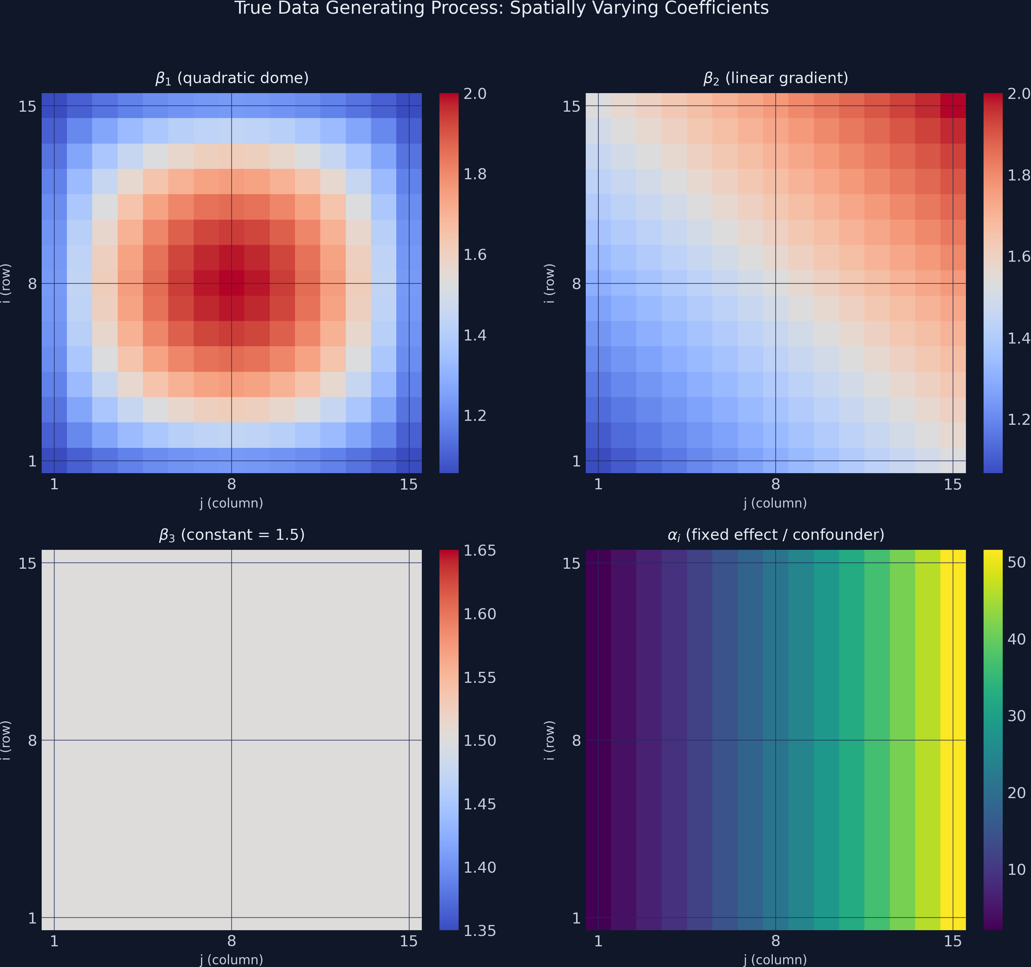
True coefficient surfaces (\(\beta_1\) dome, \(\beta_2\) gradient, \(\beta_3\) constant) versus the exponential confounder \(\alpha_i\) — which dominates the cross-section by 50× the slope range.

Spoiler figure. Don’t explain every panel yet — just plant that the confounder alpha (lower-right) has a range of ~50 units while every true slope varies by at most 1 unit. Any model that cannot separate alpha from the slopes will let it leak into the coefficient surfaces. We earn the fix in Act II.

Where we’re going

• The lab: a 225-unit, 3-period panel where place drives every covariate
• Why the naive pooled fit gets the most-biased slope backwards
• MGWFER’s one move — the within-transformation — and why it works
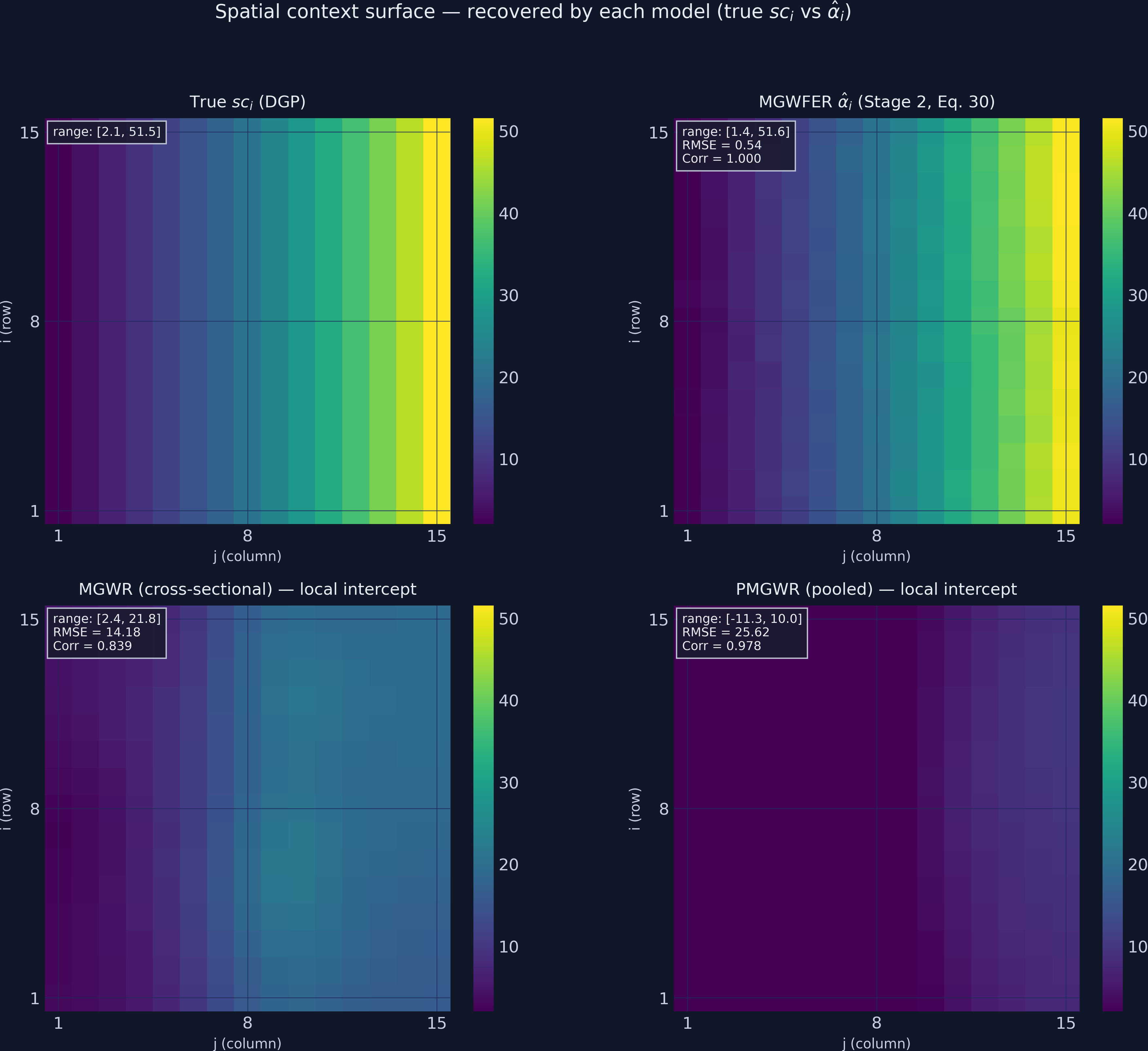
• Stage 2: recovering the confounder itself as a per-unit quantity

The Investigation

Act II

The lab: 225 spatial units × 3 periods, with place wired into every covariate

• Outcome — \(y_{it}\) built from three causally-active slopes plus a fixed effect
• Confounder — \(sc_i\) (the spatial context), exponential, range \(2\) to \(52\)
• Covariates — each one coupled to place: \(x_{k}=0.05\,sc_i+\nu_k\)

We simulate the paper’s DGP (Eqs. 39–45) verbatim on a 15×15 grid. The coupling makes the indirect channel \(sc\to x_k\) active — that is the whole point.

675 observations total. beta_1 is a quadratic dome (1.06–2.00), beta_2 a linear gradient, beta_3 constant at 1.5, beta_4 identically zero. alpha_i = 30(exp(j/15)−1). The smaller grid (vs the paper’s 30×30) keeps three bandwidth searches under ~15 minutes while exercising every step.

Couple every covariate to place and \(x_4\) correlates 0.84 with \(y\) — with zero causal effect

Quantity	Value	Meaning
\(\mathrm{Cor}(x_k, sc)\)	0.84	every covariate tracks place
\(\mathrm{Cor}(x_4, y)\)	0.84	spurious — \(\beta_4\equiv 0\)

A regression that does not condition on \(sc\) will read this 0.84 as a real effect. That is the bias mechanism, made concrete.

With sigma_x = 0.5 and 0.05·sc where sc spans 2–52, the deterministic place component dominates the noise — Cor ≈ 0.84 for all four covariates. x_4 has no causal role, yet shares the common parent sc with y, so it inherits a 0.84 correlation. This is a textbook spurious correlation through a common cause.

Wooldridge in one line: OLS recovers \(\beta_k+\delta_k\), not \(\beta_k\)

\[y = \beta_0 + \textstyle\sum_k x_k\beta_k + sc + \varepsilon, \qquad sc = \delta_0 + \textstyle\sum_k x_k\delta_k + \eta\]

\[\Rightarrow\quad y = (\beta_0+\delta_0) + \textstyle\sum_k x_k(\beta_k+\delta_k) + (\varepsilon+\eta)\]

Hide \(sc\) in the error and project it on the covariates: the bias on each slope is exactly \(\delta_k\), the indirect contextual effect.

Adapted from Wooldridge (2010, 65–67) and Eqs. 4–8 in the paper. sc is unobservable, so it folds into the error. Because sc has a linear projection on the x’s (that’s the coupling), OLS or MGWR recovers beta_k + delta_k. The magnitude of the bias is the magnitude of the indirect contextual effect. Kill delta_k and you restore identification.

Six estimators, escalating discipline — only one removes the confounder

• OLS / pooled OLS — global, no fix; the bias is on full display
• Individual FE — global, within-transform; clean but no surface
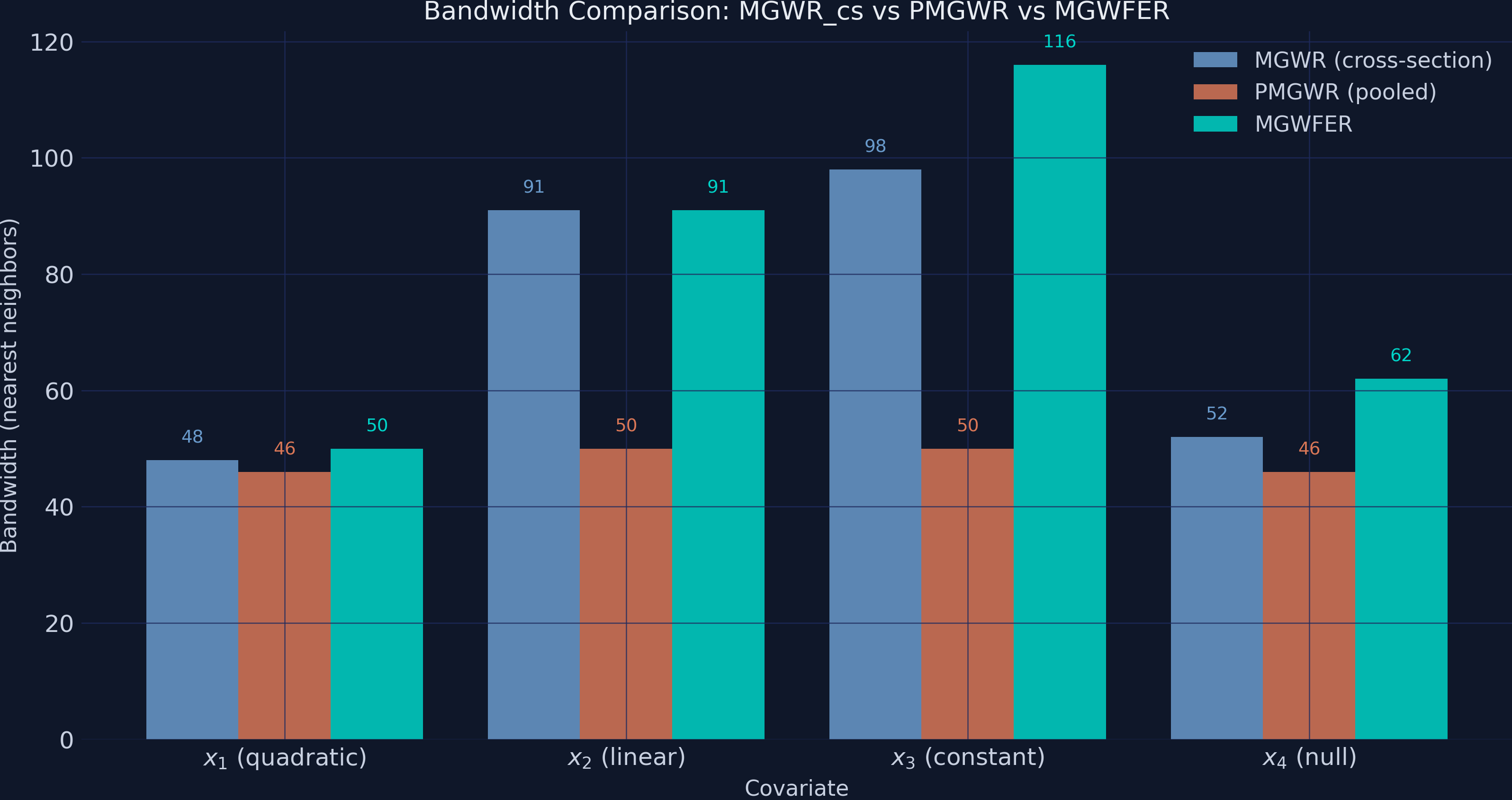
• MGWR (cross-section) / PMGWR — local surfaces, still contaminated
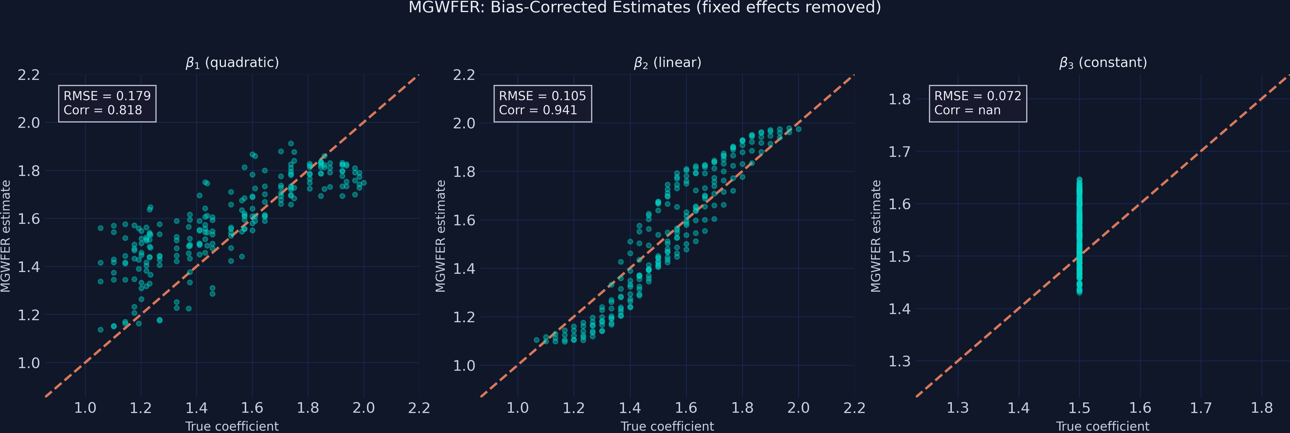
• MGWFER — local surfaces and clean identification

Only MGWFER inherits the FE estimator’s identification while delivering a location-specific coefficient surface.

The lineup mirrors the paper’s full Table 2 / Table 3. The narrative arc is escalating discipline: global naive → global FE → local naive → local FE. MGWFER is the one cell in this 2×2 (global/local × naive/FE) that has both surfaces and identification.

Globally, OLS overstates every slope ~4× and “detects” a null effect at \(p<10^{-13}\)

Coefficient	TRUE	Pooled OLS	Individual FE
\(\beta_1\)	1.50	6.14***	1.57***
\(\beta_3\)	1.50	5.79***	1.55***
\(\beta_4\)	0.00	4.16***	0.02 n.s.

OLS has nowhere to put \(sc\) except into the slopes — Wooldridge’s \(\hat\beta_k=\beta_k+\delta_k\). The within-transform neutralises it.

The paper’s Table 2 on one screen. OLS and pooled OLS estimate the true 1.5 slopes at ~6 and declare a significant beta_4 ≈ 4.2 even though beta_4 is zero. Individual FE recovers 1.57, 1.55, and beta_4 ≈ 0.02 (p = 0.66), and reconstructs mean(alpha) to within 0.06 of truth. Identification restored — but FE gives one number per coefficient, not a map.

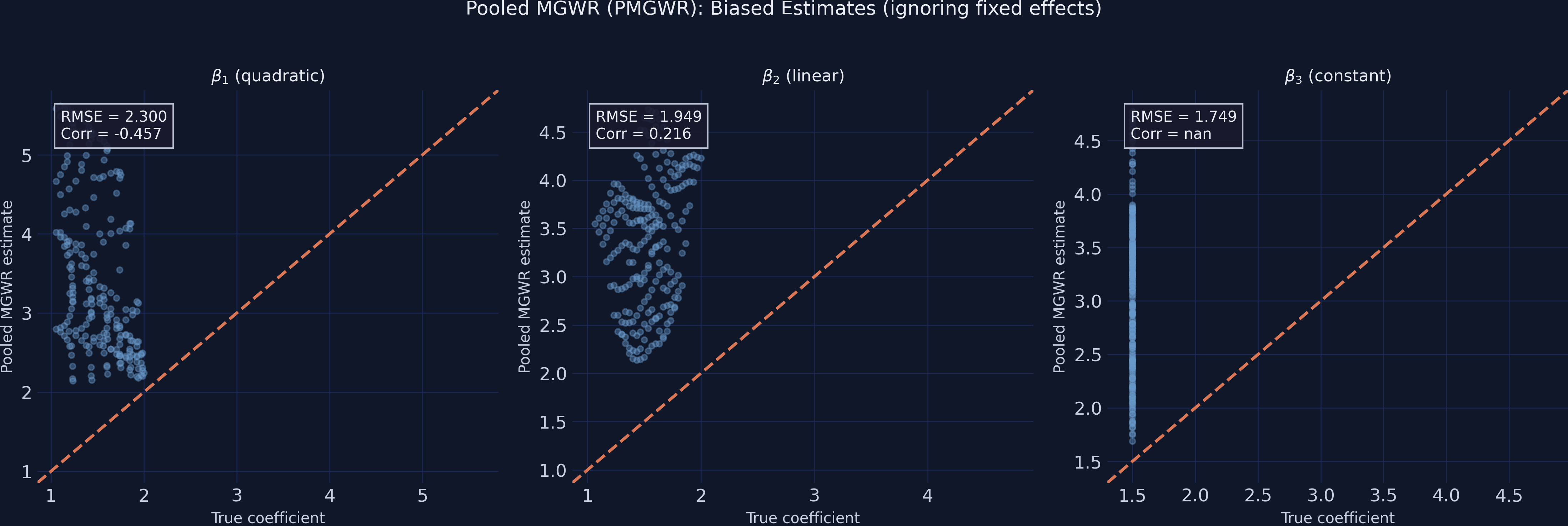
PMGWR’s local fit looks great (\(R^2=0.99\)) but \(\hat\beta_1\) is anti-correlated with truth

True vs PMGWR slopes: \(\beta_1\) scatters away from the 45° line and is anti-correlated (\(\mathrm{Cor}=-0.46\)); \(\beta_2,\beta_3\) sit well above identity.

The pooled MGWR R² of 0.989 is a trap: the local intercept (bandwidth 44) absorbs sc’s cross-sectional variation, inflating fit while the slopes go wrong. beta_1’s correlation with truth is −0.46 — the dome pattern is inverted, worse than a constant guess. A high R² fit to raw y, dominated by the confounder, tells you nothing about the slopes.

MGWFER’s one move: subtract each unit’s mean, and the confounder vanishes exactly

\[\tilde{y}_{it} = y_{it} - \bar{y}_i = \textstyle\sum_k \beta_k(u_i,v_i)\,(x_{k,it}-\bar{x}_{k,i}) + (\varepsilon_{it}-\bar\varepsilon_i)\]

Since \(\alpha_i\) is the same in every period, \(\alpha_i-\alpha_i=0\) — demeaning cancels it to machine precision.

Like zeroing a kitchen scale: subtract the container’s weight (\(\alpha_i\)) so only the contents (the slopes) remain.

The workhorse of panel econometrics. After demeaning, the max unit mean is 7e-15 — numerically exact removal. What remains is within-unit variation driven only by the spatially varying slopes and noise. The key causal assumption: no time-varying confounders (strict exogeneity conditional on the fixed effects).

Demeaning shrinks the outcome’s range from 61 to 14 — the confounder was most of the signal

• Raw \(y\) range: \([-4.07,\ 57.41]\) — spread of \(\approx 61\)
• Demeaned \(\tilde y\) range: \([-6.88,\ 6.92]\) — spread of \(\approx 14\)
• The confounder spanned \([2.07,\ 51.55]\) — and is now gone

Most of the original variation was between units. Demeaning isolates the within-unit signal that identifies the slopes.

This slide makes the within/between split concrete. Five-sixths of the raw spread lived between units, carried by alpha. Once it’s removed, what’s left is the part of y that moves over time inside one unit — exactly the variation the spatially varying coefficients explain.

Six lines fit MGWFER Stage 1 — demean, standardise, MGWR with no intercept

from mgwr.gwr import MGWR; from mgwr.sel_bw import Sel_BW
um = panel_df.groupby("unit_id")[cols].transform("mean")  # unit means
y_w, X_w = y - um["y"], X - um[xcols]                       # within-transform
sel = Sel_BW(coords, std(y_w), std(X_w), multi=True,
             constant=False, time=N_TIME)                   # no intercept
mgwfer = MGWR(coords, std(y_w), std(X_w), sel, constant=False).fit()

constant=False is load-bearing: demeaning already removed the intercept, so we fit slopes only. Standardise before the multiscale bandwidth search, then back-transform coefficients to the original scale via Eq. 29 (multiply by sigma_y_demeaned / sigma_x_k). The custom mgwr fork (GeoZhipengLi/MGWPR) adds the panel time parameter.

After demeaning, \(\hat\beta_1\)’s correlation with truth flips from \(-0.46\) to \(+0.82\)

True vs MGWFER slopes: \(\beta_1\) now clusters tightly along the 45° line (\(\mathrm{Cor}=+0.82\)); \(\beta_2,\beta_3\) collapse onto identity.

The same scatter as two slides ago, after the within-transform. beta_1 goes from getting the dome backwards to aligning with truth. RMSE drops ~92–96% for every coefficient. The within-transformation removed the very thing that contaminated the bandwidth search — everything downstream is now estimating the right surface.

RMSE falls 92–96% on every coefficient — and the sign flips on the worst one

−92%

\(\beta_1\) RMSE \(2.30\to 0.18\) vs PMGWR; correlation with truth \(-0.46\to +0.82\) (a sign reversal)

The Act-III hinge stated as one number. Not a 50% improvement, not a 2× improvement — a 10× to 25× reduction in RMSE across all four slopes, plus a sign reversal on the most-biased one. beta_2: 1.95→0.11 (−95%). beta_3: 1.75→0.07 (−96%). beta_4: 1.86→0.14 (−92%).

The Resolution

Act III

Stage 2 hands back the confounder itself — recovered at correlation 0.9996

\[\hat\alpha_i = \bar y_i - \textstyle\sum_{k} \hat\beta_{bwk}(u_i,v_i)\,\bar x_{ik}\]

Once the slopes are clean, the leftover per-unit mean is the intrinsic contextual effect — no longer a nuisance, now an output.

In MGWR the role of place hid inside one intercept; in MGWFER it is explicit, per-unit, and significance-testable.

Eq. 30 of the paper. Take each unit’s mean outcome, subtract the contribution of its mean covariates at the local slopes; what’s left is the unmeasured place effect. The derivation parallels the textbook FE result with location-specific slopes substituted for the global beta.

MGWFER reconstructs the confounder surface; PMGWR inverts it, MGWR_cs compresses it

Spatial-context surface (paper Fig. 5): true (top-left), MGWFER \(\hat\alpha_i\) near-identical (top-right), MGWR_cs compressed to \([2,22]\), PMGWR inverted to \([-11,10]\).

MGWFER’s recovered surface is visually indistinguishable from truth: range [1.45, 51.62] vs true [2.07, 51.55], correlation 0.9996, RMSE 0.54 on a 50-unit scale. MGWR_cs captures the shape (Corr 0.84) but compresses magnitude 2.5×. PMGWR’s intercept inverts and shifts negative. The paper concludes traditional local methods substantially underestimate the influence of spatial context — reproduced verbatim.

Recovered \(\hat\alpha_i\) correlates 0.9996 with the truth — every one of 225 units significant

0.9996

Pearson correlation of \(\hat\alpha_i\) with true \(sc_i\); RMSE 0.54 on a 2–52 scale; 225/225 units significant at 5%

Essentially perfect recovery. The per-unit t-test (Eqs. 32–37, df = NT − K − N = 675 − 4 − 225 = 446) flags all 225 units significant, as it should — sc_i is strictly positive everywhere. This is the deliverable no other model in the lineup can produce: per-location, significance-testable intrinsic contextual effects.

Only MGWFER reads the true process scales — PMGWR collapses every bandwidth to 44–50

Bandwidths by covariate: PMGWR flattens all to 44–50; MGWFER differentiates [50, 91, 116, 62], the largest on the spatially-constant \(\beta_3\).

Under the indirect channel every covariate looks like a noisy proxy for sc, so PMGWR picks the same small bandwidth for all of them. MGWFER recovers true process scales: small for the local dome (beta_1, bw 50), large for the spatially-constant beta_3 (bw 116). This replicates paper Table 3 — only the estimator that removes the confounder before the bandwidth search recovers the right scales.

The strongest objection — does the within-transform make this causal?

Objection. Demeaning only removes time-invariant confounders — a one-trick pony. Real places change.

Response. True. MGWFER removes time-invariant confounding cleanly — and only that. It does not manufacture identification.

Steelman, don’t strawman. Identification rests on four assumptions: time-invariant sc, strict exogeneity, no time-varying confounders, and stable slopes. The within-transformation deals with time-invariant confounding only; any unobserved factor that changes over time and correlates with both x and y still biases MGWFER. Time-invariant measurable covariates (e.g. distance to highway) get swept into alpha_hat and are no longer separable — a structural property of FE estimators. Be honest about the boundary.

The stakes are real: on Georgia data, MGWFER flips poverty’s sign and 10× the place effect

MGWR / PMGWR

• intrinsic effect \(\approx\pm 0.3\) (\(\pm 1.5\%\))
• poverty coefficient: positive
• “role of place” looks small

MGWFER

• intrinsic effect \(\approx\pm 4\) (\(\pm 20\%\))
• poverty coefficient: negative
• place effect \(10\times\) larger

The paper’s Georgia case study (159 counties, 2016–2020 ACS, bachelor’s-degree share). Conventional MGWR finds a positive poverty–education link with no defensible causal reading; MGWFER reverses it to negative, in line with prior literature, and recovers intrinsic contextual effects an order of magnitude larger. The bias is not academic — it changes the policy story.

Let the within-transformation, not the bandwidth search, decide what place is doing.

The single takeaway. Remove the time-invariant confounder before the spatial smoother runs, and two things happen at once: the local slopes become identified (−0.46 → +0.82) and the confounder itself becomes a clean, per-unit, testable output (r = 0.9996). One move; two payoffs.