Double Machine Learning with 401(k) Data

From eligibility effects to complier analysis

$8,730DML ATE of eligibility

55%naive gap that was bias

$11,746IIVM LATE on compliers

Carlos Mendez

Nagoya University (GSID)

July 8, 2026

The Tension

Act I

Eligible households hold $19,559 more — but is the 401(k) the cause?

Over $7 trillion sits in U.S. 401(k) accounts. Eligible households hold $19,559 more in net financial assets than ineligible ones.

But eligible households also earn $15,368 more income. Is the gap the plan — or the people who get the plan?

This is the central question of the tutorial. The raw eligibility gap of $19,559 is the kind of number a press release quotes. Our job over the next 18 slides is to find out how much of it is the causal effect of access and how much is confounding — chiefly income. Policymakers expanding 401(k) eligibility need the causal part, not the press-release part.

One dataset, three models, very different answers

Naive baselines (gray) versus three DML models across four ML learners, \(\hat\theta \pm 95\%\) CI. Naive overstates; DML cuts it roughly in half.

Spoiler figure — plant it now, earn it in Act II. Don’t explain every bar yet. Just note the two gray naive bars sit far to the right of everything else, the steel (PLR) and orange (IRM) bars cluster together around $8,000–$9,000, and the teal (IIVM) bars sit higher because they answer a different question. We return to this picture in the Resolution.

Where we’re going

• The confounding problem: why naive comparisons mislead
• The DML recipe: orthogonal scores + cross-fitting
• Three estimands — PLR & IRM (ATE), IIVM (LATE)
• Four ML learners — and why the answer barely moves
• The lesson: separate “is it real?” from “for whom?”

Agenda built from the post’s learning objectives. Teaching deck, so we signpost the arc once and then follow it.

The Investigation

Act II

The lab: 9,915 households from the 1991 SIPP survey

• Outcome \(Y\) — net total financial assets (net_tfa), median just $1,499
• Treatment \(D\) — 401(k) eligibility (e401), 37.1% eligible
• Endogenous treatment — actual participation (p401), 26.2%
• Controls \(X\) — 9 covariates: income, age, education, family size, and 5 more

Eligibility is set by the employer; participation is a household choice. That distinction drives all three models.

9,915 U.S. households. The outcome is wildly skewed — median $1,499, mean $18,052, range from −$502,302 to $1,536,798. About 70% of eligible households actually enroll. The eligibility-vs-participation split is the hinge of the whole deck: eligibility is plausibly exogenous after conditioning on X; participation is a choice tangled up with unobserved financial discipline.

Income drives both access and savings — the textbook confounder

Eligible households (blue) earn far more and cluster in the high-income, high-wealth region. Income opens a backdoor path from access to savings.

Left panel: the income distributions barely overlap — eligible households average $46,862 versus $31,494, a $15,368 gap. Right panel: blue (eligible) points pile into the upper-right. This is exactly the pattern a naive comparison conflates with a causal effect. Comparing 401(k) holders to non-holders is like crediting gym memberships for fitness: the people who join were already different.

The naive estimate is the causal effect plus confounding bias

\[\hat\Delta_{\text{naive}} = \underbrace{\theta_0}_{\text{causal effect}} + \underbrace{\text{bias}}_{\text{income, education, }\ldots}\]

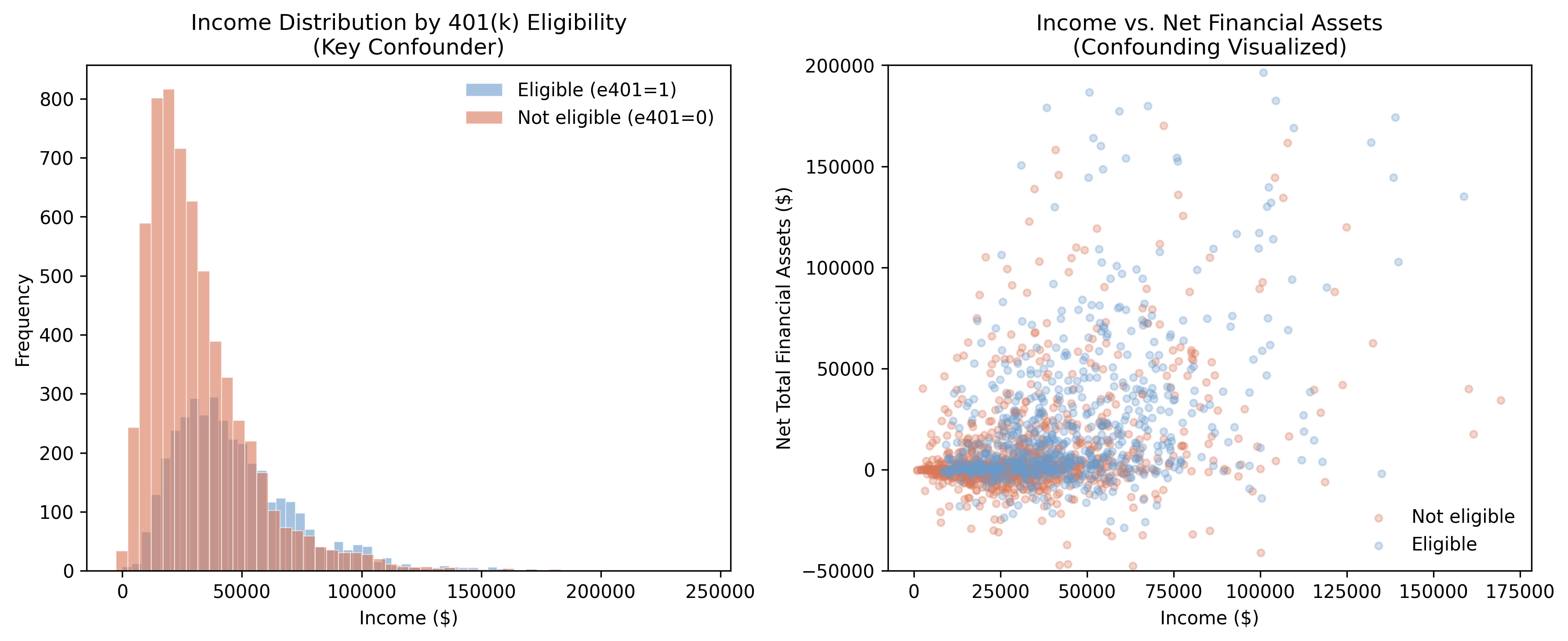
The naive $19,559 is not wrong arithmetic — it is the right gap answering the wrong question. DML’s whole job is to subtract the second term.

The naive difference-in-means is a clean number that confuses two things. Decompose it: the true causal effect we want, plus all pre-existing differences between the groups. Standard linear regression can subtract some bias, but only if the confounding is linear. When income-to-savings curves nonlinearly, linear adjustment leaves bias behind. That is the gap ML fills.

DML strips the confounding with two nuisance functions

\[Y = \theta_0 D + g_0(X) + \varepsilon, \qquad D = m_0(X) + V\]

\(g_0(X) = E[Y\mid X]\)

Predict savings from covariates. Residual \(\tilde Y = Y - \hat g_0(X)\) is the unexplained savings.

\(m_0(X) = E[D\mid X]\)

Predict eligibility from covariates. Residual \(\tilde D = D - \hat m_0(X)\) is the surprise eligibility.

Regress \(\tilde Y\) on \(\tilde D\): the slope is \(\hat\theta_0\). Both residuals are cleaned of confounding, so only the causal channel remains.

Think noise-cancelling headphones: the ML models learn the confounding “noise” pattern and subtract it; the clean causal signal is what’s left. This is partialling out — the same logic as Frisch–Waugh–Lovell, but with flexible learners instead of OLS, so it captures nonlinear confounding. Crucially θ comes from the unshrunk residual-on-residual regression, never from a shrunk ML coefficient.

Two safeguards make ML-based nuisance estimation harmless

Neyman-orthogonal score

The estimating equation’s derivative w.r.t. small nuisance errors is zero at the truth. Sloppy \(\hat g_0, \hat m_0\) barely move \(\hat\theta_0\).

Cross-fitting (K-fold)

Fit \(\hat g_0, \hat m_0\) on \(K-1\) folds, predict on the held-out fold, rotate. No row is ever scored by a model that saw it.

Orthogonality kills regularization bias; cross-fitting kills overfitting bias. Together they let Lasso, forests, or XGBoost serve as nuisance learners with no harm to inference.

This is the engine of the whole method. The orthogonal (doubly-robust) score is built so first-order nuisance errors cancel — that is why we can plug in biased, regularized ML estimates. Cross-fitting is the rotating-judge trick: each fold’s residuals come from a model that never saw that fold, so a flexible learner can’t memorize quirks and manufacture artificially clean residuals. Remove either safeguard and the inference breaks.

Six lines fit a DML model in Python

import doubleml as dml
data_dml = dml.DoubleMLData(data, y_col="net_tfa", d_cols="e401", x_cols=features_base)

ml_l = RandomForestRegressor(...)   # g0: outcome nuisance
ml_m = RandomForestClassifier(...)  # m0: treatment nuisance

model = dml.DoubleMLPLR(data_dml, ml_l=ml_l, ml_m=ml_m, n_folds=3)
model.fit()                          # cross-fitting + orthogonal score, internally

The DoubleML package hides all the rotation and orthogonalization. You declare the data roles (Y, D, X, and later Z), pick two learners, choose the number of folds, and call fit(). The library cross-fits and applies the orthogonal score behind the scenes — no manual train/test commands. We swap ml_l / ml_m to test robustness across four learners.

PLR: a constant-effect ATE of $8,730 — less than half the naive gap

PLR estimates across four ML learners; all cluster near $8,000–$9,400, far below the $19,559 naive line (dashed).

PLR assumes one constant treatment effect θ0 and lets the controls enter g0 flexibly. Estimates run $7,823 (Decision Tree) to $9,371 (Lasso), mean $8,730. Versus the naive $19,559, DML reveals roughly $10,829 — 55% — was confounding bias. Every 95% CI excludes zero. The range across learners is just $1,548: the answer barely depends on which ML algorithm you pick, which is the robustness hallmark of DML.

IRM relaxes the constant-effect assumption — and lands at $8,213

\[\theta_0 = E\!\left[g_0(1,X) - g_0(0,X) + \frac{D\,(Y-g_0(1,X))}{m_0(X)} - \frac{(1-D)\,(Y-g_0(0,X))}{1-m_0(X)}\right]\]

The doubly-robust (AIPW) score: an outcome model corrected by inverse-propensity weighting. Consistent if either \(g_0\) or \(m_0\) is right — a safety net.

IRM drops PLR’s additivity. It combines an outcome model g0(D,X) with a propensity score m0(X) = P(D=1|X) into the doubly-robust score above. “Doubly robust” = consistent if either model is correct, not necessarily both. Propensity weighting upweights informative rare controls — an “eligible-type” household that wasn’t eligible is the cleanest counterfactual. Trimming at 0.01 drops extreme propensity scores so the IPW weights stay stable.

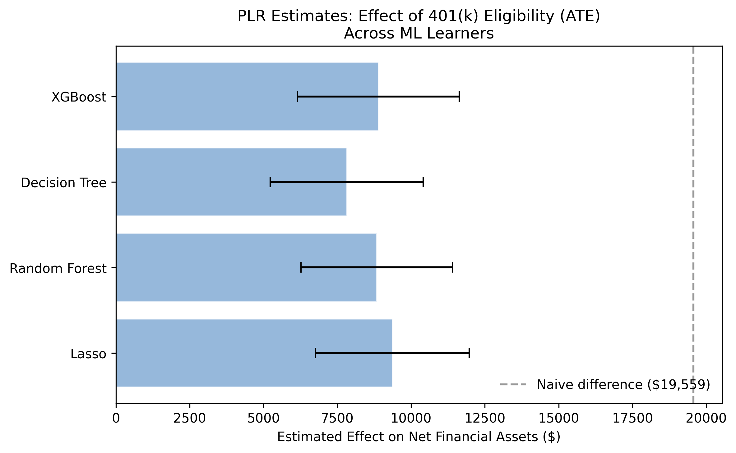
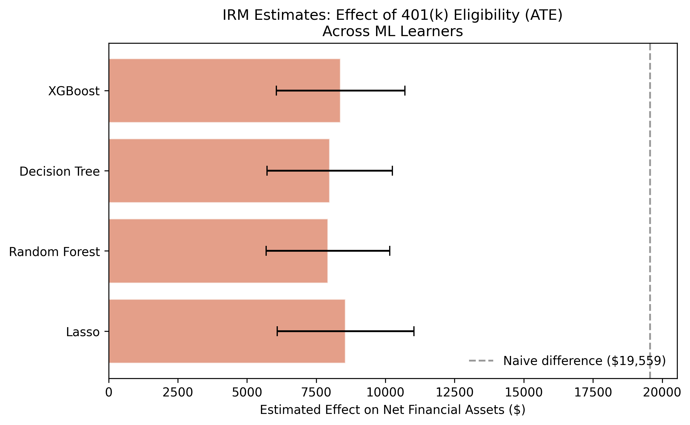
Two different recipes, same answer: PLR and IRM agree within $517

IRM estimates across four learners ($7,924–$8,559) are even tighter than PLR, with smaller standard errors.

IRM mean is $8,213 — only $517 below PLR’s $8,730. This convergence is the payoff of running both: partialling-out (PLR) and doubly-robust AIPW (IRM) rest on different assumptions and combine nuisances differently, yet they agree the ATE is $8,000–$9,000. That agreement means the number isn’t an artifact of one modeling choice. IRM’s SEs are even a touch smaller ($1,185 vs $1,339), so the propensity approach is slightly more efficient here. The close agreement also signals limited effect heterogeneity.

Participation is a choice — so we instrument it with eligibility

\[\theta_{\text{LATE}} = \frac{E[Y\mid Z=1] - E[Y\mid Z=0]}{E[D\mid Z=1] - E[D\mid Z=0]}\]

Participation \(D\) is endogenous (financial discipline is unobserved). Eligibility \(Z\) is a nudge: it opens the door without forcing anyone through.

A Wald-type ratio: the instrument’s effect on savings, divided by its effect on participation.

PLR and IRM estimate the effect of eligibility, which is plausibly exogenous given X. But the effect of actually participating is endogenous — the enroll/don’t-enroll choice is driven by unobserved traits (financial literacy, savings motivation) that also drive savings. IIVM uses eligibility as an instrument for participation: relevance (you can’t participate without being eligible) plus exclusion (eligibility affects savings only through participation, given X). The estimand it recovers is the LATE.

The instrument only moves the compliers — so the LATE is their effect

Type	Behavior	In the LATE?
Always-takers	Participate regardless of eligibility	no
Never-takers	Never participate, even if eligible	no
Compliers	Participate because eligible	yes
Defiers	Assumed not to exist (monotonicity)	—

The LATE is the effect of participation on the marginal households a policy actually moves.

Eligibility flips the participation status of compliers only. Always-takers would save in IRAs or taxable accounts anyway; never-takers won’t enroll no matter what. The instrument doesn’t move them, so they’re not in the estimate. That’s why the LATE is “local” — it’s the effect for exactly the population an eligibility expansion targets. Defiers are ruled out by the monotonicity assumption.

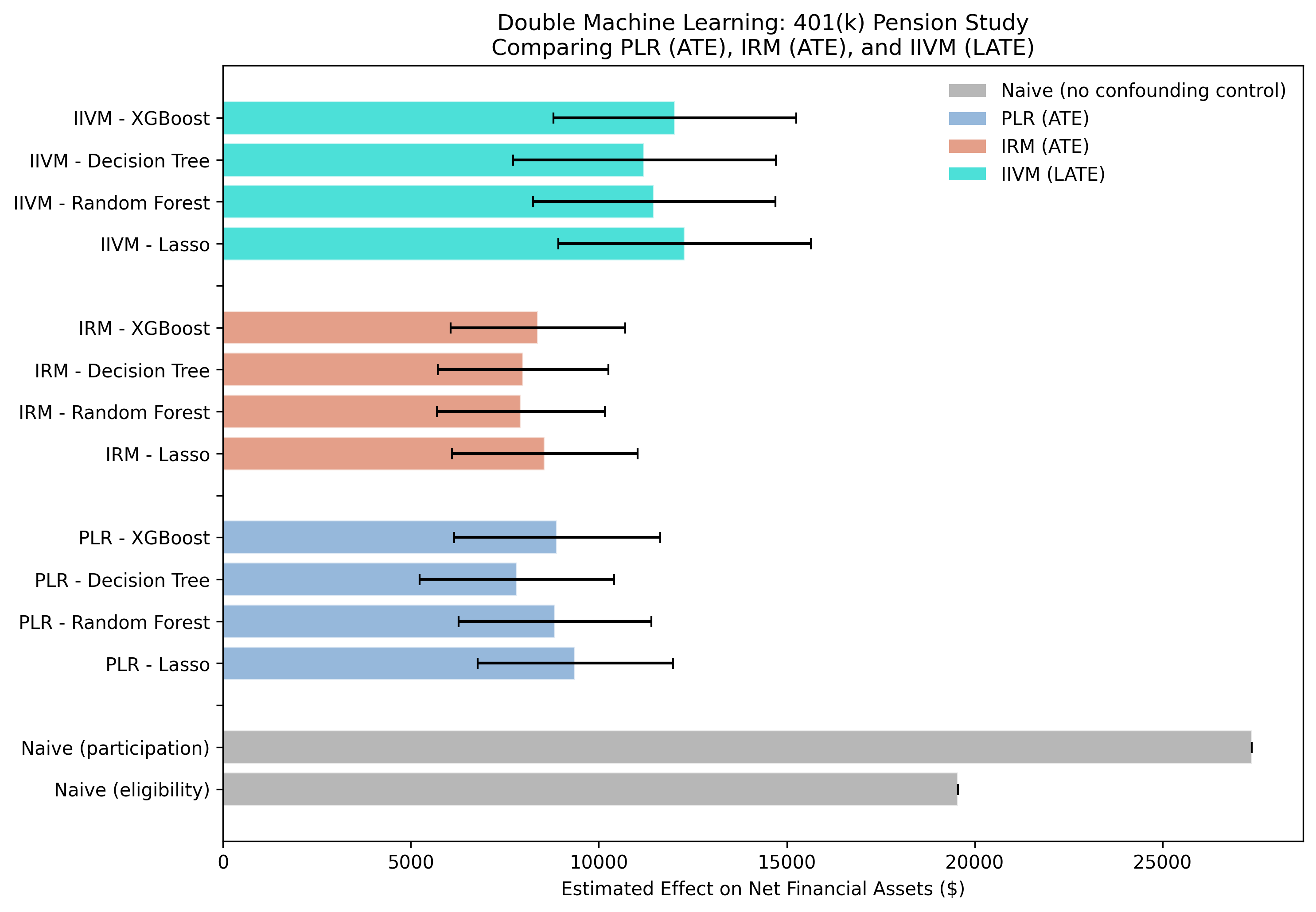
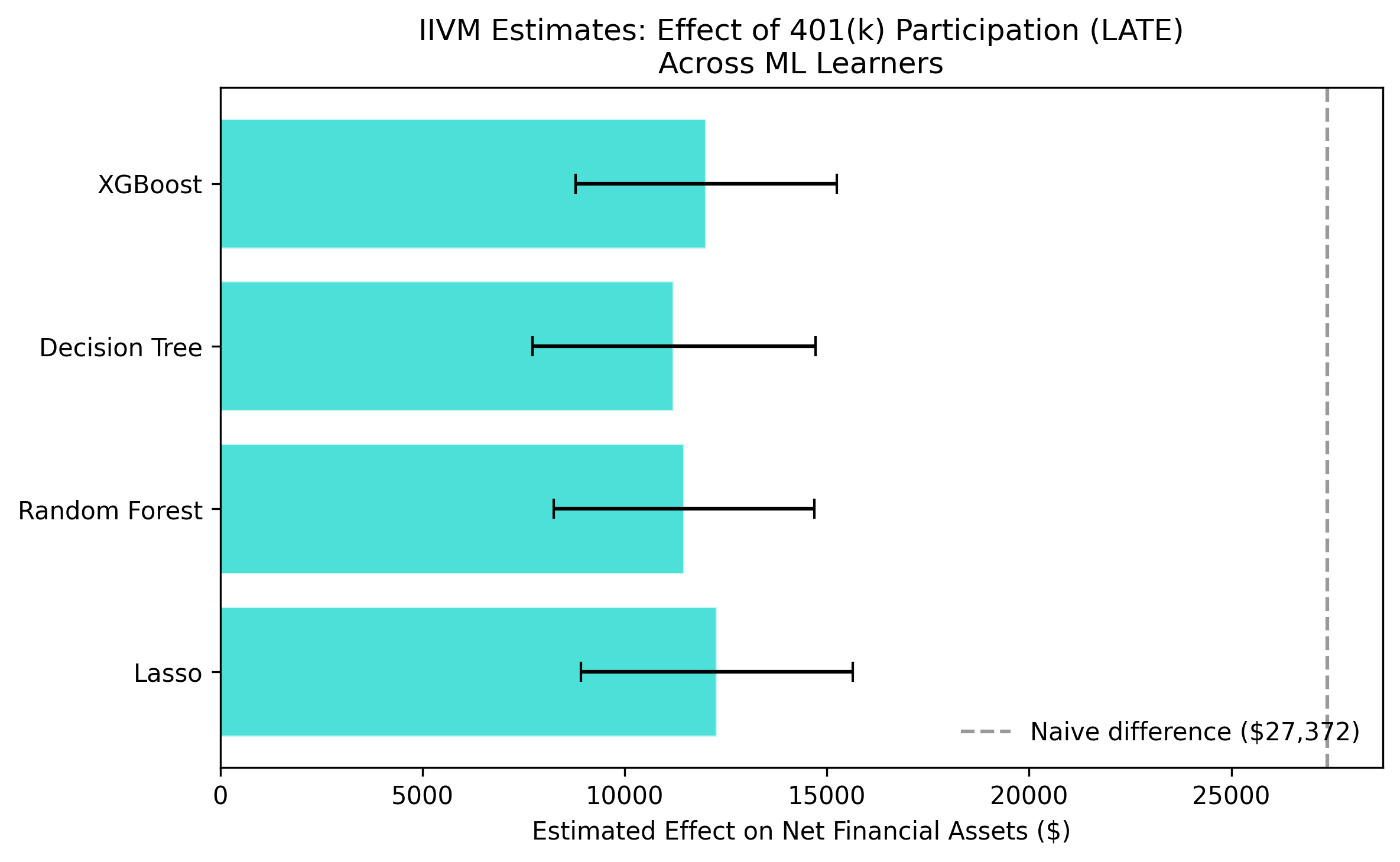
The IIVM LATE is $11,746 — larger than the ATE, by design

IIVM LATE estimates across four learners ($11,215–$12,281) sit well above the ATE band, as expected for compliers.

The LATE runs $11,215 to $12,281, mean $11,746 — about 35% above the $8,000–$8,700 ATE. Not a contradiction: a different estimand. Compliers are marginal participants whose savings behavior genuinely changes with access, so the 401(k) channels new savings rather than reshuffling existing wealth. SEs are larger ($1,698 avg) — the efficiency cost of IV — but every estimate stays significant. The whole IV machinery still rides on cross-fitting and the orthogonal score.

Estimates barely move across four learners — orthogonality at work

Whole-picture comparison: naive (gray), PLR (steel), IRM (orange), IIVM (teal). Within each model the four learners cluster tightly.

Back to the spoiler — now earned. Within-model spread is tiny: $1,548 for PLR, $635 for IRM, $1,066 for IIVM. Lasso, Random Forest, Decision Tree, and XGBoost plug into the same orthogonal score and give nearly the same answer. That insensitivity to the nuisance learner is precisely what Neyman orthogonality buys you — the first-order nuisance error cancels, so the choice of ML algorithm is second-order.

The Resolution

Act III

55% of the naive eligibility gap was pure confounding bias

55%

of the $19,559 naive gap (≈ $10,829) was income-driven bias, not causal effect — the ATE is $8,730

The headline of the whole analysis. The naive eligibility estimate of $19,559 overstates the true ATE by 124%. DML attributes roughly $10,829 — 55% — to confounding, chiefly the $15,368 income gap. What survives, $8,730, is the genuine causal effect of access. More than half of the press-release number was an illusion.

Eligibility genuinely raises savings — about $8,500 per household

$8,730

PLR mean ATE (IRM: $8,213); every 95% CI across two models and four learners excludes zero

After debiasing, the effect is smaller but real and robust. Two distinct DML frameworks (PLR and IRM) and four ML learners all land in the $8,000–$9,400 range, and not a single confidence interval touches zero. For a policymaker: each newly eligible household can be expected to accumulate roughly $8,500 more in net financial assets, on average.

For the households a policy actually moves, the effect is $12,000

$11,746

IIVM LATE on compliers — the marginal participants an eligibility expansion targets

The ATE answers “what’s the average effect?”; the LATE answers “what’s the effect for the people a new policy moves?” Newly eligible households are compliers by definition, so for the target population of an eligibility expansion the relevant number is closer to $12,000 than $8,500. ATE and LATE aren’t rivals — they answer different policy questions.

Does DML make this causal? No — two assumptions still carry the weight

Objection. Letting an ML model pick the controls can’t manufacture identification.

Response. Correct. DML disciplines estimation, not identification.

The ATE needs conditional exogeneity; the LATE adds instrument validity and monotonicity.

Steelman, don’t strawman. DML’s contribution is honest, efficient estimation given identification — not identification itself. The ATE is identified only under conditional exogeneity of eligibility given X; the LATE adds instrument validity and monotonicity. Flexible nuisances plus orthogonality plus cross-fitting discipline estimation, but they do not relax the identifying assumptions — if financial literacy confounds eligibility and savings, the estimates stay biased. Conditional exogeneity is untestable; the IV exclusion restriction is an assumption, not a result. The 1991 SIPP is also a single cross-section, and extreme asset outliers (−$502k to +$1.5M) pull the mean-based ATE. The method is a microscope, not a randomizer.

Separate “is the effect real?” from “for whom?” — and let cross-fitting do the rest.

The single takeaway. PLR and IRM answer “is it real, and how big on average?” — $8,730, with 55% of the naive gap exposed as bias. IIVM answers “for whom does it matter most?” — $11,746 for the compliers a policy moves. Across both, the orthogonal score plus cross-fitting make four very different ML learners agree. That is double machine learning earning its name.